Quantitative Analysis in R
Session 2 · Hypothesis Testing
2026-07-26
Welcome back
- Session 1: describing data — means, SDs, grouped summaries, plots
- Session 2 (today): moving from description to inference
- is an observed difference/relationship likely real, or just chance?
- Four core tests: t-test, ANOVA, correlation test, chi-square
Session 2 roadmap
| Time | Topic |
|---|---|
| 0–10 min | From description to inference: what a p-value means |
| 10–30 min | Comparing two groups: t.test() |
| 30–50 min | Comparing 3+ groups: ANOVA |
| 50–70 min | Testing relationships: correlation & chi-square |
| 70–90 min | Your Turn: choose the right test + wrap-up |
From Description to Inference
What a p-value actually means
- Null hypothesis (H₀): no real difference/relationship exists in the population; anything we see in our sample is due to chance
- A p-value is the probability of seeing a difference this large or larger, if H₀ were true
- Small p-value (conventionally < 0.05) → the data would be unusual under H₀ → we reject H₀
What a p-value is not: it is not the probability that H₀ is true, and it is not the probability your result is “important.” A tiny p-value can come from a trivial effect if the sample is large enough — always report the effect size alongside it.
The general workflow for every test today
- State H₀ (no difference/relationship) and H₁ (there is one)
- Check the test’s assumptions (visually, from Session 1 skills)
- Run the test in R
- Read the p-value and the effect size / confidence interval
- Write one sentence of plain-language interpretation
Comparing Two Groups
Independent-samples t-test
Question: does body mass differ between male and female penguins?
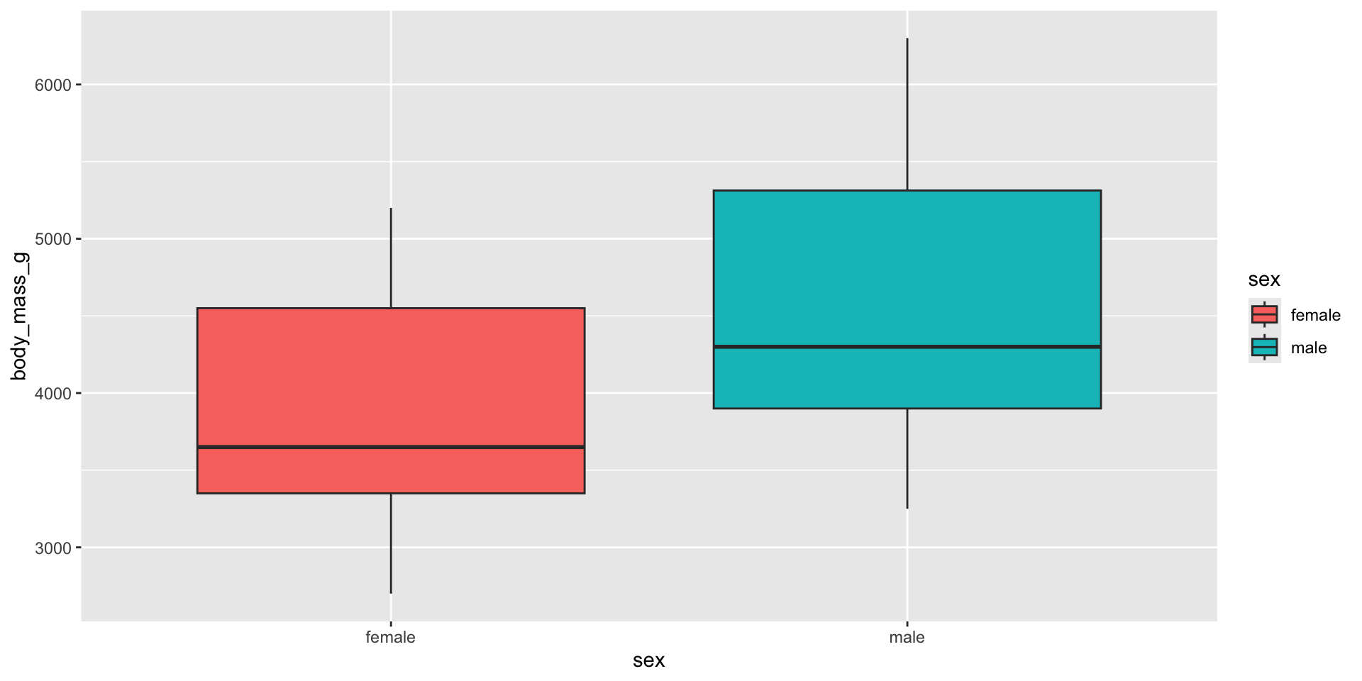
Always look first — a large visible difference with non-overlapping boxes is a strong hint before we even run the test.
Running the t-test
    Welch Two Sample t-test

data:  body_mass_g by sex
t = -8.5545, df = 323.9, p-value = 4.794e-16
alternative hypothesis: true difference in means between group female and group male is not equal to 0
95 percent confidence interval:
 -840.5783 -526.2453
sample estimates:
mean in group female   mean in group male
            3862.273             4545.685
Reading the output:
t= test statistic,df= degrees of freedomp-value— here, extremely small → strong evidence of a real difference- 95% confidence interval — the likely range for the true difference in means
- Reports means for each group at the bottom
Checking assumptions
- t-test assumes roughly normal distributions and (for the default
t.test()) does not assume equal variances (Welch’s correction is used automatically) - Quick normality check: histogram, or
shapiro.test()for a formal test
    Shapiro-Wilk normality test

data:  pull(filter(penguins, sex == "male"), body_mass_g)
W = 0.92504, p-value = 1.227e-07
With large samples, shapiro.test() often flags “non-normal” even for minor deviations — visual inspection (histogram/QQ-plot) is usually more useful in practice than the formal test alone.
Your Turn 1 (8 min)
Test whether flipper_length_mm differs by sex.
- Boxplot first
- Run
t.test() - Write one sentence interpreting the result
Answer
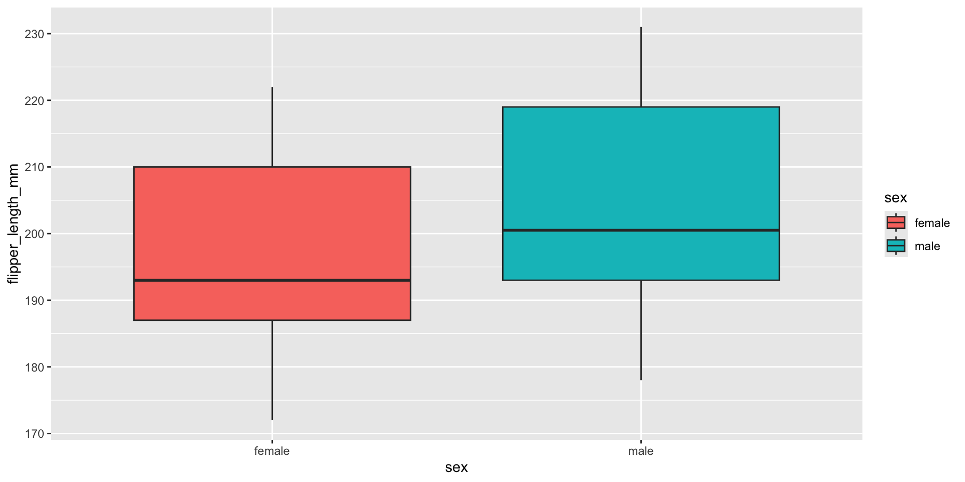
    Welch Two Sample t-test

data:  flipper_length_mm by sex
t = -4.8079, df = 325.28, p-value = 2.336e-06
alternative hypothesis: true difference in means between group female and group male is not equal to 0
95 percent confidence interval:
 -10.064811  -4.219821
sample estimates:
mean in group female   mean in group male
            197.3636             204.5060
“Male penguins have significantly longer flippers than female penguins (p < .001).”
Comparing Three or More Groups
One-way ANOVA
Question: does body mass differ across the three species?
             Df    Sum Sq  Mean Sq F value Pr(>F)
species       2 145190219 72595110   341.9 <2e-16 ***
Residuals   330  70069447   212332
---
Signif. codes:  0 '***' 0.001 '**' 0.01 '*' 0.05 '.' 0.1 ' ' 1
ANOVA tests whether at least one group differs from the others — it does not tell you which pair(s) differ. The significant Pr(>F) here says species matters, but we need a follow-up test to know which species differ from which.
Post-hoc test: Tukey HSD
  Tukey multiple comparisons of means
    95% family-wise confidence level

Fit: aov(formula = body_mass_g ~ species, data = penguins)

$species
                       diff       lwr       upr    p adj
Chinstrap-Adelie   26.92385 -132.3528  186.2005 0.916431
Gentoo-Adelie    1386.27259 1252.2897 1520.2554 0.000000
Gentoo-Chinstrap 1359.34874 1194.4304 1524.2671 0.000000
Every pairwise comparison, with an adjusted p-value that corrects for multiple testing. Reading the output: adelie-Gentoo, Adelie-Chinstrap, Chinstrap-Gentoo — check the p adj column for each pair.
Checking ANOVA assumptions visually
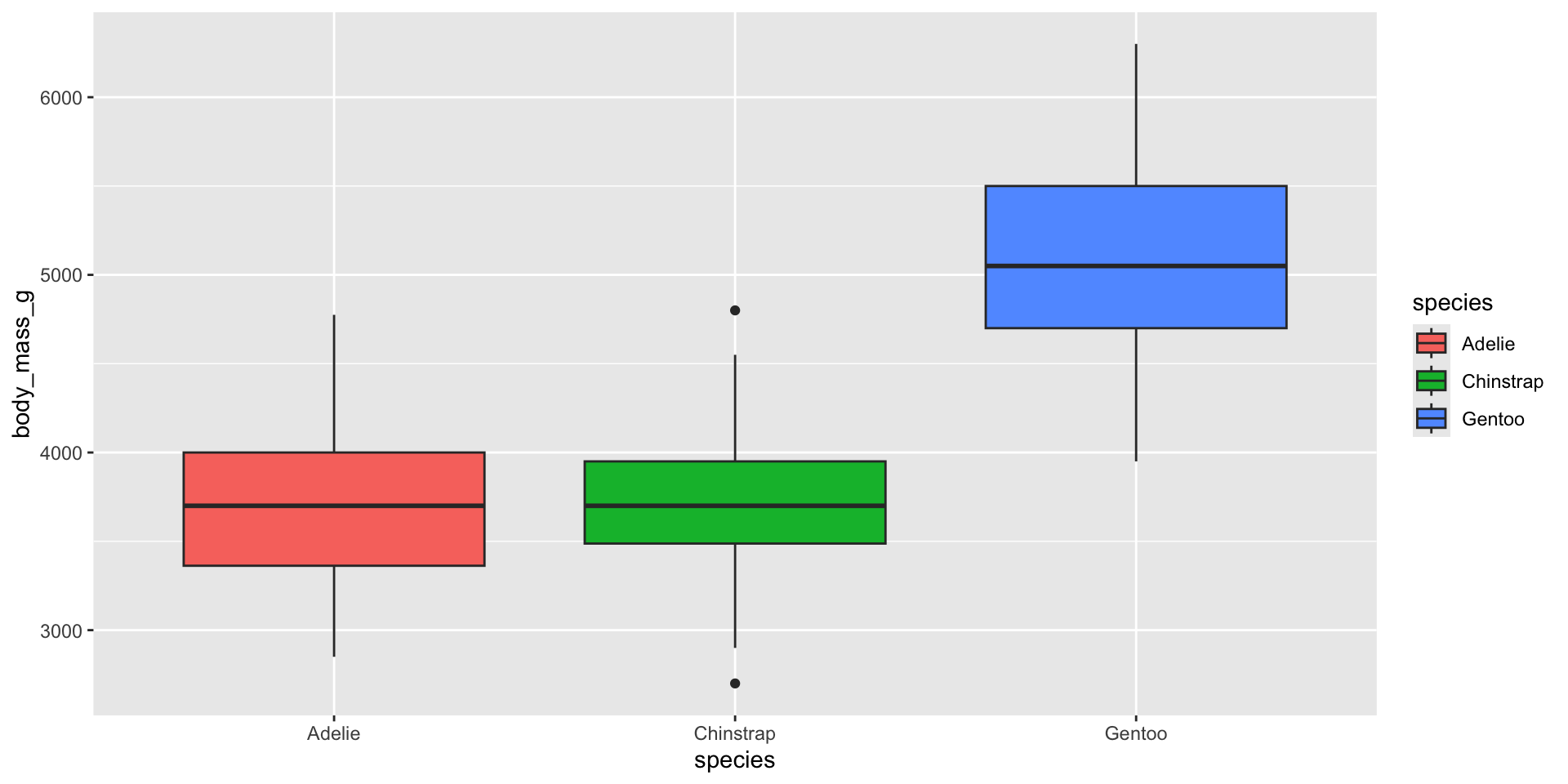
Roughly similar spread across groups (homogeneity of variance) and roughly symmetric boxes (approximate normality) — both look reasonable here.
Your Turn 2 (10 min)
- Run an ANOVA testing whether
flipper_length_mmdiffers byspecies - Run
TukeyHSD()on it - Which species pairs differ significantly?
Answer
             Df Sum Sq Mean Sq F value Pr(>F)
species       2  50526   25263   567.4 <2e-16 ***
Residuals   330  14693      45
---
Signif. codes: 0 '***' 0.001 '**' 0.01 '*' 0.05 '.' 0.1 ' ' 1 Tukey multiple comparisons of means
95% family-wise confidence level
Fit: aov(formula = flipper_length_mm ~ species, data = penguins)
$species
diff lwr upr p adj
Chinstrap-Adelie 5.72079 3.414364 8.027215 0
Gentoo-Adelie 27.13255 25.192399 29.072709 0
Gentoo-Chinstrap 21.41176 19.023644 23.799885 0All three pairwise comparisons are significant — every species differs from every other in flipper length.
Testing Relationships
Correlation test
    Pearson's product-moment correlation

data:  penguins$bill_length_mm and penguins$flipper_length_mm
t = 15.691, df = 331, p-value < 2.2e-16
alternative hypothesis: true correlation is not equal to 0
95 percent confidence interval:
 0.5868092 0.7106869
sample estimates:
      cor
0.6530956
Compare to Session 1’s plain cor() — now we get a p-value and confidence interval alongside the correlation coefficient (cor in the output), telling us whether this relationship is distinguishable from zero.
Chi-square test of independence
Question: is species associated with island?
            Biscoe Dream Torgersen
  Adelie        44    55        47
  Chinstrap      0    68         0
  Gentoo       119     0         0
    Pearson's Chi-squared test

data:  tbl
X-squared = 284.59, df = 4, p-value < 2.2e-16
Chi-square tests whether two categorical variables are independent. Here, the tiny p-value confirms what we already suspected visually in Session 1 — species and island are strongly associated (Torgersen = Adelie only, etc.).
Your Turn 3 (10 min)
- Test the correlation between
bill_depth_mmandbody_mass_gwithcor.test() - Build a table of
speciesbysexand run a chi-square test — are they associated?
Answer
    Pearson's product-moment correlation

data:  penguins$bill_depth_mm and penguins$body_mass_g
t = -9.741, df = 331, p-value < 2.2e-16
alternative hypothesis: true correlation is not equal to 0
95 percent confidence interval:
 -0.5515130 -0.3840214
sample estimates:
       cor
-0.4720157
            female male
  Adelie        73   73
  Chinstrap     34   34
  Gentoo        58   61
    Pearson's Chi-squared test

data:  tbl2
X-squared = 0.048607, df = 2, p-value = 0.976
Species and sex are not significantly associated (roughly equal male/female split within each species) — a good example of a non-significant, and equally informative, result.
Choosing the Right Test
A quick decision guide
| Question | Variable types | Test |
|---|---|---|
| Do 2 groups differ? | 1 numeric + 1 categorical (2 levels) | t.test() |
| Do 3+ groups differ? | 1 numeric + 1 categorical (3+ levels) | aov() + TukeyHSD() |
| Are two numeric variables related? | 2 numeric | cor.test() |
| Are two categorical variables associated? | 2 categorical | chisq.test() |
Your Turn 4 — Final Practice (10 min)
For each research question below, state which test you’d use, then run it:
- Does
bill_length_mmdiffer betweenislands(3 levels)? - Is there a relationship between
bill_length_mmandbill_depth_mm?
Answer
             Df Sum Sq Mean Sq F value   Pr(>F)
island        2   1417   708.6   27.47 9.21e-12 ***
Residuals   330   8512    25.8
---
Signif. codes:  0 '***' 0.001 '**' 0.01 '*' 0.05 '.' 0.1 ' ' 1
# Q2: 2 numeric variables -> correlation test
cor.test(penguins$bill_length_mm, penguins$bill_depth_mm)
    Pearson's product-moment correlation

data:  penguins$bill_length_mm and penguins$bill_depth_mm
t = -4.2726, df = 331, p-value = 2.528e-05
alternative hypothesis: true correlation is not equal to 0
95 percent confidence interval:
 -0.3280409 -0.1242017
sample estimates:
       cor
-0.2286256
Recap — Session 2
- A p-value tells you how surprising your data would be if there were truly no effect — not the probability the effect is real or important
t.test()— two groups;aov()+TukeyHSD()— three or more groupscor.test()— relationship between two numeric variables;chisq.test()— association between two categorical variables- Always visualise first, check assumptions, and report effect size/CI alongside the p-value
Before Session 3
Practice at home:
Next session: regression — quantifying how much one variable predicts another, and how to report model results in a paper-ready way.
Thank you!
Session 2 complete
SARA Institute of Data Science
SARA Institute of Data Science · Quantitative Analysis in R