Quantitative Analysis in R

Session 3 · Regression & Reporting Results

SARA Institute of Data Science

2026-07-25

Welcome back

Session 1: describing data · Session 2: testing whether differences/relationships are real
Session 3 (today): regression — quantifying how much a variable predicts another, and reporting results properly
Ends with a mini project: full describe → test → model → report workflow

Session 3 roadmap

Time	Topic
0–15 min	Simple linear regression
15–40 min	Multiple regression
40–60 min	Model diagnostics
60–80 min	Reporting results with `broom`
80–90 min	Mini project + wrap-up

Simple Linear Regression

From correlation to regression

Session 2’s cor.test() told us whether flipper_length_mm and body_mass_g are related, and how strongly
Regression goes further: it gives us an equation to predict one from the other

model1 <- lm(body_mass_g ~ flipper_length_mm, data = penguins)
summary(model1)


Call:
lm(formula = body_mass_g ~ flipper_length_mm, data = penguins)

Residuals:
     Min       1Q   Median       3Q      Max 
-1057.33  -259.79   -12.24   242.97  1293.89 

Coefficients:
                  Estimate Std. Error t value Pr(>|t|)    
(Intercept)       -5872.09     310.29  -18.93   <2e-16 ***
flipper_length_mm    50.15       1.54   32.56   <2e-16 ***
---
Signif. codes:  0 '***' 0.001 '**' 0.01 '*' 0.05 '.' 0.1 ' ' 1

Residual standard error: 393.3 on 331 degrees of freedom
Multiple R-squared:  0.7621,    Adjusted R-squared:  0.7614 
F-statistic:  1060 on 1 and 331 DF,  p-value: < 2.2e-16

Reading the output

summary(model1)

Intercept: predicted body_mass_g when flipper_length_mm = 0 (often not meaningful on its own)
Slope (flipper_length_mm coefficient): for every 1mm increase in flipper length, body mass increases by this many grams
p-value (per coefficient): is this slope distinguishable from zero?
R-squared: proportion of variance in body_mass_g explained by flipper_length_mm (0 to 1)

Visualising the fitted line

ggplot(penguins, aes(x = flipper_length_mm, y = body_mass_g)) +
  geom_point(alpha = 0.5) +
  geom_smooth(method = "lm", se = TRUE) +
  labs(title = "Body Mass Predicted by Flipper Length")

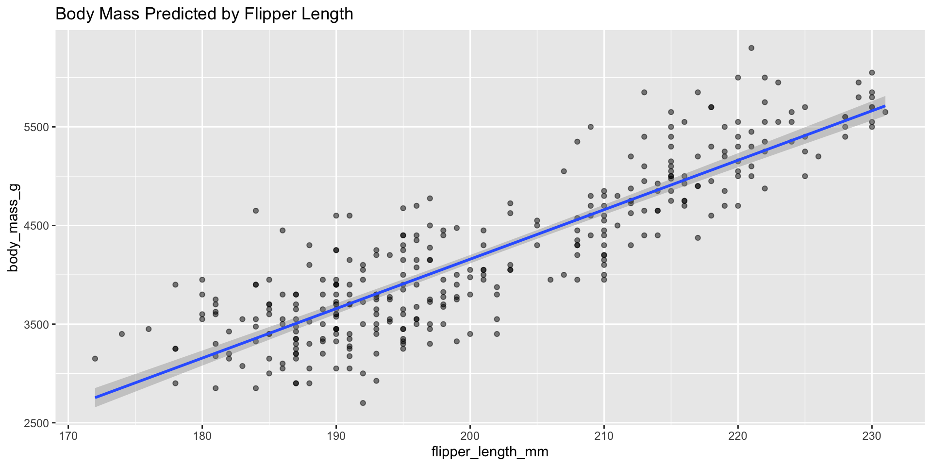
geom_smooth(method = "lm") — the exact line lm() just fit for you, with its confidence band.

Your Turn 1 (10 min)

Fit lm(bill_length_mm ~ bill_depth_mm, data = penguins)
What is the slope? Is it significant?
What is the R²? How much variance is explained?

Answer

model_yt1 <- lm(bill_length_mm ~ bill_depth_mm, data = penguins)
summary(model_yt1)


Call:
lm(formula = bill_length_mm ~ bill_depth_mm, data = penguins)

Residuals:
     Min       1Q   Median       3Q      Max 
-12.9498  -3.9530  -0.3657   3.7327  15.5025 

Coefficients:
              Estimate Std. Error t value Pr(>|t|)    
(Intercept)    54.8909     2.5673  21.380  < 2e-16 ***
bill_depth_mm  -0.6349     0.1486  -4.273 2.53e-05 ***
---
Signif. codes:  0 '***' 0.001 '**' 0.01 '*' 0.05 '.' 0.1 ' ' 1

Residual standard error: 5.332 on 331 degrees of freedom
Multiple R-squared:  0.05227,   Adjusted R-squared:  0.04941 
F-statistic: 18.26 on 1 and 331 DF,  p-value: 2.528e-05

The slope is negative and significant here — but recall Session 1’s warning about Simpson’s Paradox: this ignores species, which we’ll fix next.

Multiple Regression

Adding more predictors

model2 <- lm(body_mass_g ~ flipper_length_mm + species + sex, data = penguins)
summary(model2)


Call:
lm(formula = body_mass_g ~ flipper_length_mm + species + sex, 
    data = penguins)

Residuals:
   Min     1Q Median     3Q    Max 
-721.8 -195.7   -5.9  198.6  873.7 

Coefficients:
                  Estimate Std. Error t value Pr(>|t|)    
(Intercept)       -365.817    532.050  -0.688   0.4922    
flipper_length_mm   20.025      2.846   7.037 1.15e-11 ***
speciesChinstrap   -87.634     46.347  -1.891   0.0595 .  
speciesGentoo      836.260     85.185   9.817  < 2e-16 ***
sexmale            530.381     37.810  14.027  < 2e-16 ***
---
Signif. codes:  0 '***' 0.001 '**' 0.01 '*' 0.05 '.' 0.1 ' ' 1

Residual standard error: 295.6 on 328 degrees of freedom
Multiple R-squared:  0.8669,    Adjusted R-squared:  0.8653 
F-statistic:   534 on 4 and 328 DF,  p-value: < 2.2e-16

Categorical predictors (species, sex) are automatically converted to dummy variables — one level becomes the reference category (shown by what’s missing from the output, e.g. Adelie and female)
Each coefficient is now interpreted holding the other variables constant: “controlling for species and sex, each extra mm of flipper length predicts X more grams”

Interpreting categorical coefficients

summary(model2)

speciesChinstrap — average difference in body mass between Chinstrap and Adelie (the reference), holding flipper length and sex constant
speciesGentoo — same, for Gentoo vs. Adelie
sexmale — average difference between male and female, holding species and flipper length constant

This is the payoff of multiple regression: it separates the effect of flipper length from the effect of species — exactly the confound Simpson’s Paradox warned us about.

Comparing models: does adding predictors help?

model_simple <- lm(body_mass_g ~ flipper_length_mm, data = penguins)
model_full   <- lm(body_mass_g ~ flipper_length_mm + species + sex, data = penguins)

summary(model_simple)$r.squared

[1] 0.7620922

summary(model_full)$r.squared

[1] 0.8668884

R² increases substantially once species and sex are added — flipper length alone was leaving real, systematic variation unexplained.

Your Turn 2 (10 min)

Fit body_mass_g ~ bill_length_mm + island + sex
Which predictors are significant?
Compare its R² to the simple flipper_length_mm-only model

Answer

model_yt2 <- lm(body_mass_g ~ bill_length_mm + island + sex, data = penguins)
summary(model_yt2)


Call:
lm(formula = body_mass_g ~ bill_length_mm + island + sex, data = penguins)

Residuals:
    Min      1Q  Median      3Q     Max 
-1133.1  -263.4    63.9   315.8  1120.6 

Coefficients:
                Estimate Std. Error t value Pr(>|t|)    
(Intercept)     1747.419    231.710   7.541 4.60e-13 ***
bill_length_mm    60.616      5.249  11.547  < 2e-16 ***
islandDream     -935.736     54.081 -17.302  < 2e-16 ***
islandTorgersen -625.304     81.271  -7.694 1.69e-13 ***
sexmale          449.676     53.085   8.471 8.32e-16 ***
---
Signif. codes:  0 '***' 0.001 '**' 0.01 '*' 0.05 '.' 0.1 ' ' 1

Residual standard error: 450.6 on 328 degrees of freedom
Multiple R-squared:  0.6906,    Adjusted R-squared:  0.6868 
F-statistic:   183 on 4 and 328 DF,  p-value: < 2.2e-16

Model Diagnostics

Why check diagnostics

A high R² and significant p-values mean little if the model’s core assumptions are badly violated
Four things to check: linearity, normality of residuals, constant variance (homoscedasticity), and influential outliers

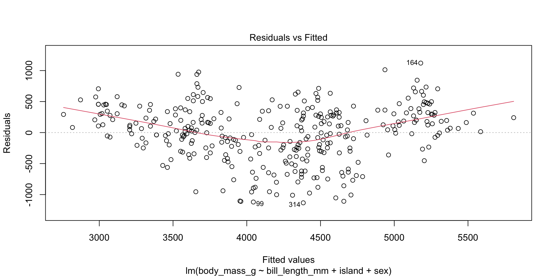
Residual plots

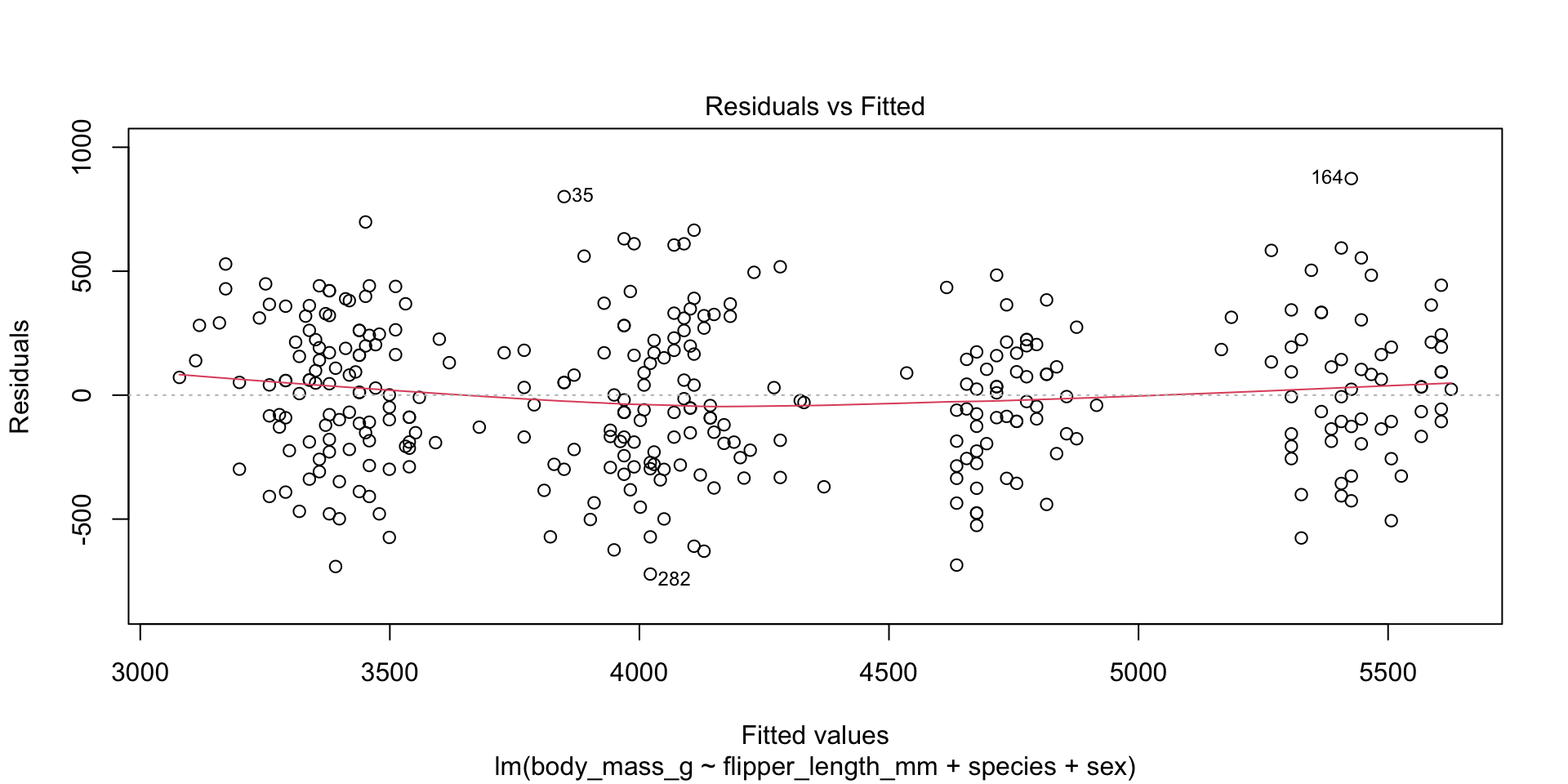
plot(model2, which = 1)  # Residuals vs Fitted

Looking for: a roughly random scatter of points around the horizontal zero line, with no funnel shape or curve. A clear pattern here would suggest a violated assumption.

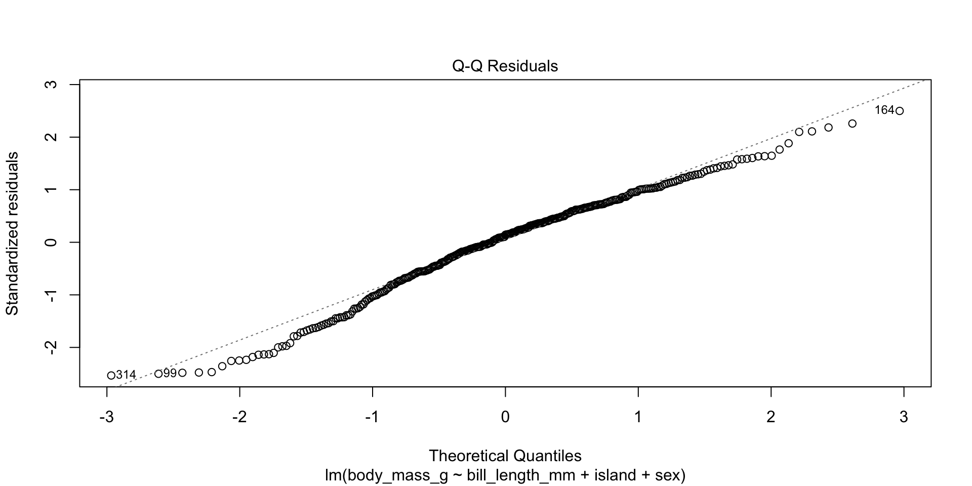
Normal Q-Q plot

plot(model2, which = 2)  # Normal Q-Q

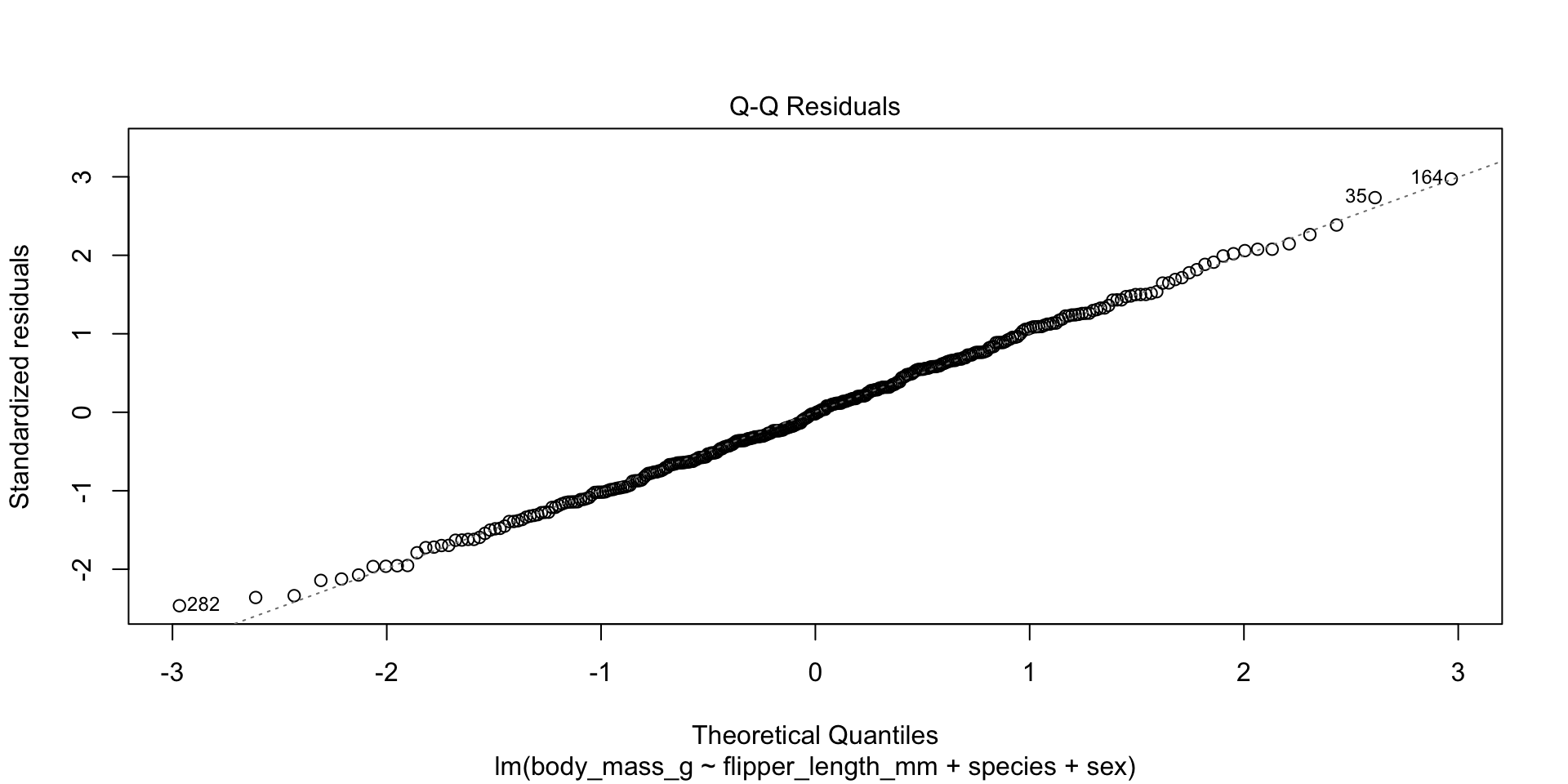
Points should fall roughly along the diagonal line. Points that stray far at the ends suggest non-normal residuals — worth investigating those specific rows.

A ggplot-based alternative

augment(model2) |>
  ggplot(aes(x = .fitted, y = .resid)) +
  geom_point(alpha = 0.5) +
  geom_hline(yintercept = 0, linetype = "dashed", color = "red") +
  labs(title = "Residuals vs Fitted Values", x = "Fitted", y = "Residual")

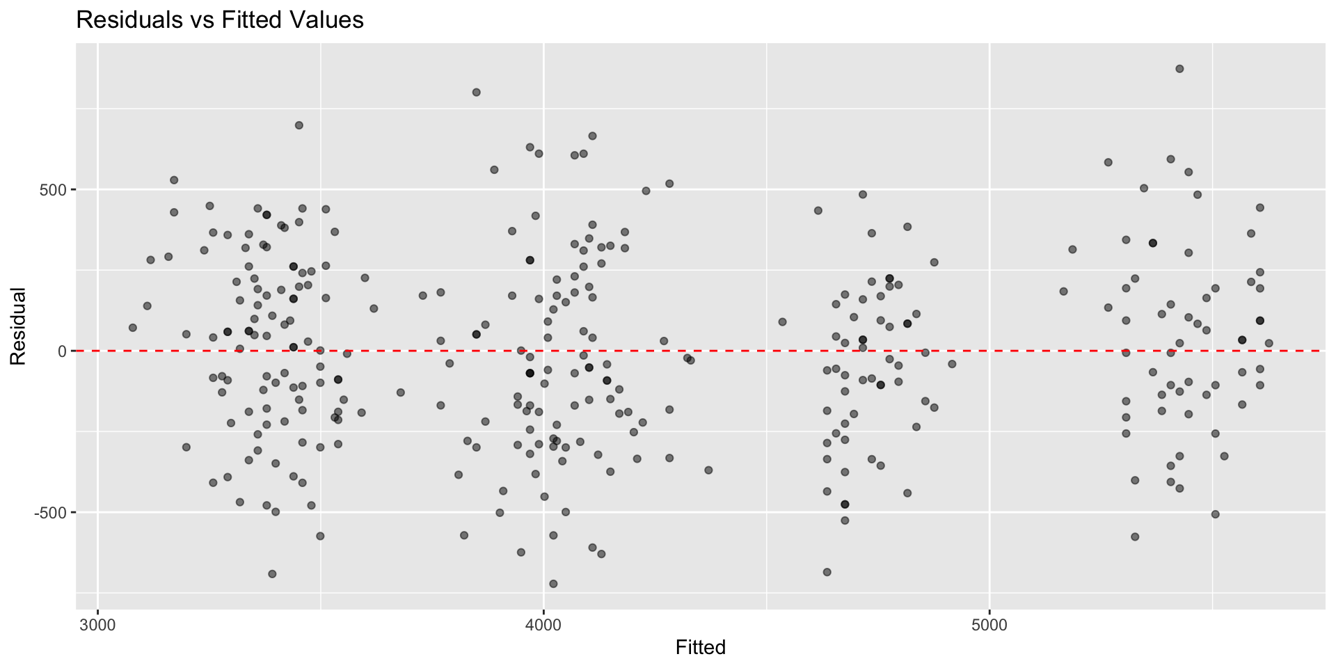
augment() from broom adds fitted values and residuals directly onto your original data — useful for diagnostics in a consistent ggplot2 workflow.

Your Turn 3 (7 min)

Run diagnostic plots (which = 1 and which = 2) on your Your Turn 2 model. Do the assumptions look reasonably satisfied?

Answer

plot(model_yt2, which = 1)

plot(model_yt2, which = 2)

Reporting Results

Tidy model output with `broom`

tidy(model2)

# A tibble: 5 × 5
  term              estimate std.error statistic  p.value
  <chr>                <dbl>     <dbl>     <dbl>    <dbl>
1 (Intercept)         -366.     532.      -0.688 4.92e- 1
2 flipper_length_mm     20.0      2.85     7.04  1.15e-11
3 speciesChinstrap     -87.6     46.3     -1.89  5.95e- 2
4 speciesGentoo        836.      85.2      9.82  4.11e-20
5 sexmale              530.      37.8     14.0   2.41e-35

Compare this to raw summary(model2) output — tidy() returns a clean data frame you can filter, sort, round, or export directly into a table for a paper or report.

Rounding and formatting for a report

tidy(model2) |>
  mutate(across(where(is.numeric), ~round(.x, 3)))

# A tibble: 5 × 5
  term              estimate std.error statistic p.value
  <chr>                <dbl>     <dbl>     <dbl>   <dbl>
1 (Intercept)         -366.     532.      -0.688   0.492
2 flipper_length_mm     20.0      2.85     7.04    0    
3 speciesChinstrap     -87.6     46.3     -1.89    0.06 
4 speciesGentoo        836.      85.2      9.82    0    
5 sexmale              530.      37.8     14.0     0

glance(model2)

# A tibble: 1 × 12
  r.squared adj.r.squared sigma statistic   p.value    df logLik   AIC   BIC
      <dbl>         <dbl> <dbl>     <dbl>     <dbl> <dbl>  <dbl> <dbl> <dbl>
1     0.867         0.865  296.      534. 3.37e-142     4 -2364. 4741. 4764.
# ℹ 3 more variables: deviance <dbl>, df.residual <int>, nobs <int>

glance() gives one-row, whole-model summary statistics (R², adjusted R², F-statistic, p-value) — exactly what typically goes in a results paragraph or a methods table.

Writing results in report-ready language

“A multiple linear regression was conducted to predict body mass from flipper length, species, and sex. The model explained a significant proportion of variance in body mass, R² = 0.87, F(4, 328) = 534, p < .001. Flipper length was a significant positive predictor (b = 20.02, p < .001), controlling for species and sex.”

Notice the sentence structure: what was tested → whether the model overall was significant (R², F, p) → what each key predictor contributed (b, p). This template works for almost any regression write-up.

Your Turn 4 (8 min)

Using your Your Turn 2 model, write one report-style sentence covering:

Overall model significance (R², p)
One specific predictor’s effect

Answer (example)

“A multiple regression predicting body mass from bill length, island, and sex explained a significant proportion of variance, R² = [value], p < .001. Sex was a significant predictor, with male penguins on average [X] grams heavier than female penguins, controlling for bill length and island.”

Mini Project

Mini project (10–15 min)

Pick one outcome variable and one research question from penguins. Complete the full workflow:

Describe: relevant summary statistics + one plot (Session 1 skills)
Test: an appropriate hypothesis test for your question (Session 2 skills)
Model: a regression with at least one numeric and one categorical predictor
Report: one paragraph combining your findings in report-ready language

Share your one paragraph with a neighbour — does it read clearly to someone who hasn’t seen your code?

Recap — all three sessions

Session 1: descriptive statistics — mean/median, SD/IQR, grouped summaries, visual exploration
Session 2: hypothesis testing — t-test, ANOVA, correlation test, chi-square, and what a p-value does (and doesn’t) mean
Session 3: regression — simple and multiple lm(), diagnostics, and reporting with broom
You now hold a complete, R-based quantitative analysis workflow: describe → test → model → report

Where to go next

Book: Discovering Statistics Using R (Andy Field) — approachable, widely used in the social sciences
Package: report — auto-generates APA-style write-ups from model objects
Practice: apply this exact workflow to your own thesis/research data
Next at SARA: consider a follow-on session on generalized linear models (logistic regression) if your data includes binary outcomes

Thank you!

All three sessions complete

SARA Institute of Data Science

Quantitative Analysis in R

Welcome back

Session 3 roadmap

Simple Linear Regression

From correlation to regression

Reading the output

Visualising the fitted line

Your Turn 1 (10 min)

Multiple Regression

Adding more predictors

Interpreting categorical coefficients

Comparing models: does adding predictors help?

Your Turn 2 (10 min)

Model Diagnostics

Why check diagnostics

Residual plots

Normal Q-Q plot

A ggplot-based alternative

Your Turn 3 (7 min)

Reporting Results

Tidy model output with broom

Rounding and formatting for a report

Writing results in report-ready language

Your Turn 4 (8 min)

Mini Project

Mini project (10–15 min)

Recap — all three sessions

Where to go next

Thank you!

Tidy model output with `broom`