Quantitative
Analysis
Theory
“Theory is a well-established principle or set of general principles to explain a broad range of observations.”
Theory = Explanation = Generalisation
Population
The population is the complete set of all individuals, items, or observations that share a common characteristic and are of interest to the researcher.
It has unknown parameters which we estimate.
Sample
A sample is a subset of the population that’s actually observed or measured in the study.
Samples have statistics
Statistical Inference
- The goal of most research is statistical inference: using sample statistics to make educated guesses about population parameters.
Variables
“Elements in the study that are measured or manipulated.”
Independent variable
Dependent variable
Statistical Learning
“Statistical Learning refers to a vast set of tools for understanding data.”
Summarizes and organizes data to describe its main features.
Limited to the observed data.
Makes predictions or inferences about a population from a sample.
Goes beyond the observed data to infer population characteristics.
Central Tendency & Spread
R Packages
Measures of central tendency
[1] 4201.754[1] 4050na.rm = TRUEis essential here — without it,mean()returnsNAif even one value is missing- Mean vs. median: mean is pulled by outliers/skew; median is more robust. Always check both, especially with real-world (messy) data
Key Insights
Mean: Best for symmetric datasets but affected by outliers.
Median: Robust to outliers, useful for skewed data.
Mode: Describes the most common value, useful for categorical data.
Skewness

Source: Wikipedia
Measures of spread
[1] 801.9545[1] 643131.1[1] 1200 0% 25% 50% 75% 100%
2700 3550 4050 4750 6300 - SD: average distance from the mean, same units as the variable
- Variance: SD squared — used more in formulas than in reporting
- IQR: range of the middle 50% — robust to outliers, pairs naturally with the median
Grouped Summaries
group_by() + summarise()
penguins |>
  group_by(species) |>
  summarise(
    mean_mass = mean(body_mass_g, na.rm = TRUE),
    sd_mass   = sd(body_mass_g, na.rm = TRUE),
    n         = n()
  )
# A tibble: 3 × 4
species mean_mass sd_mass n
<fct> <dbl> <dbl> <int>
1 Adelie 3701. 459. 152
2 Chinstrap 3733. 384. 68
3 Gentoo 5076. 504. 124This is the single most-used pattern in applied quantitative work: “give me this statistic, for each level of this category.”
Grouping by more than one variable
penguins |>
  group_by(species, sex) |>
  summarise(mean_mass = mean(body_mass_g, na.rm = TRUE), .groups = "drop")
# A tibble: 8 × 3
species sex mean_mass
<fct> <fct> <dbl>
1 Adelie female 3369.
2 Adelie male 4043.
3 Adelie <NA> 3540
4 Chinstrap female 3527.
5 Chinstrap male 3939.
6 Gentoo female 4680.
7 Gentoo male 5485.
8 Gentoo <NA> 4588..groups = "drop" avoids a message and returns a plain (ungrouped) tibble — good habit once you start chaining more steps after summarise().
Standard Error
penguins |>
  filter(!is.na(body_mass_g)) |>
  group_by(species) |>
  summarise(
    mean_mass = mean(body_mass_g),
    se_mass   = sd(body_mass_g) / sqrt(n())
  )
# A tibble: 3 × 3
species mean_mass se_mass
<fct> <dbl> <dbl>
1 Adelie 3701. 37.3
2 Chinstrap 3733. 46.6
3 Gentoo 5076. 45.5SD describes spread of individual penguins. Standard error (SE) describes uncertainty in the mean itself — how much would this mean likely shift if we resampled?
Visual Exploration
Why visualise before testing
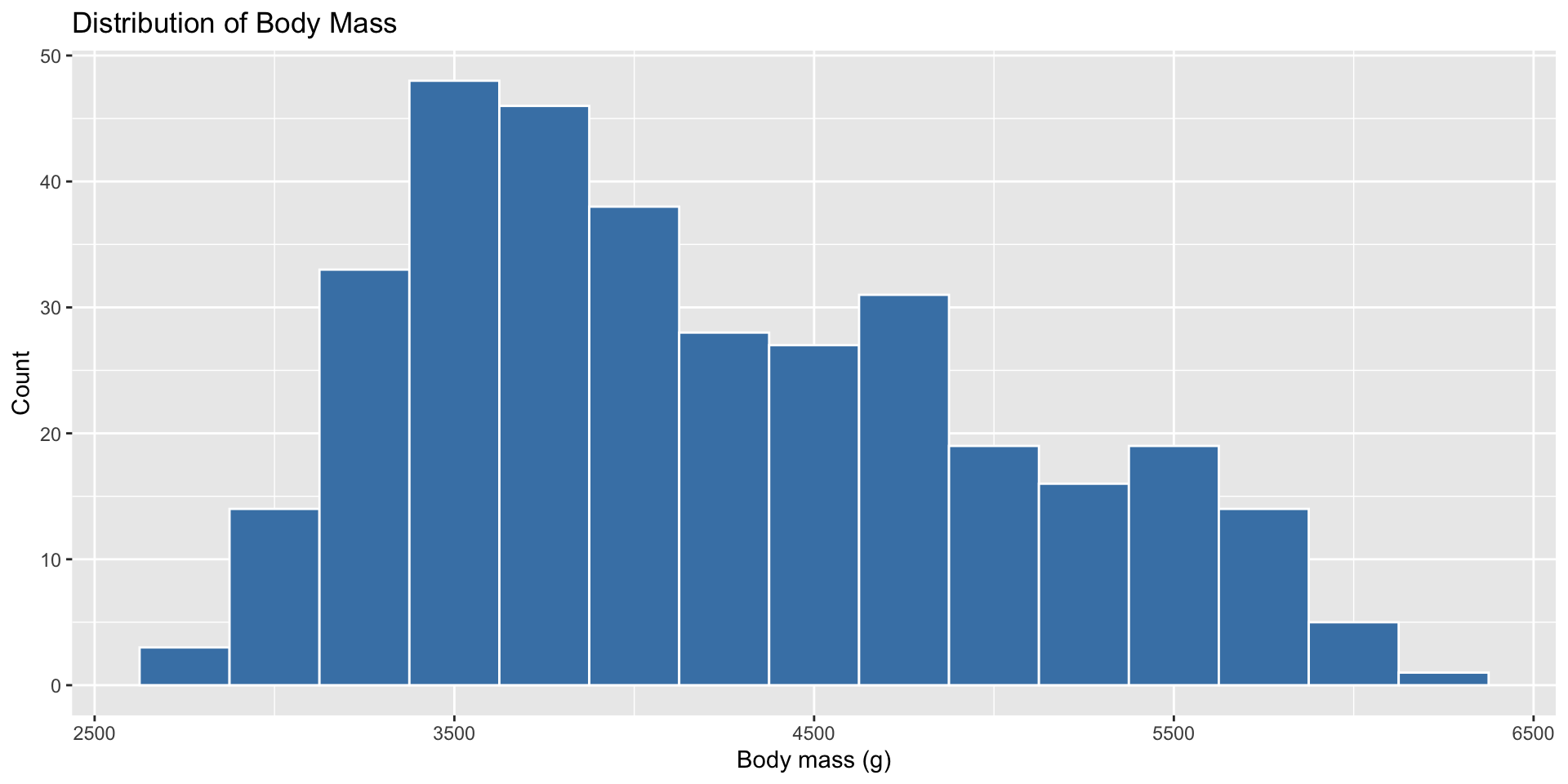
- Numbers alone can hide skew, outliers, or multi-modal distributions
- A quick plot often prevents a wrong statistical choice later (e.g. running a t-test on badly skewed data)
Histogram — shape of one variable
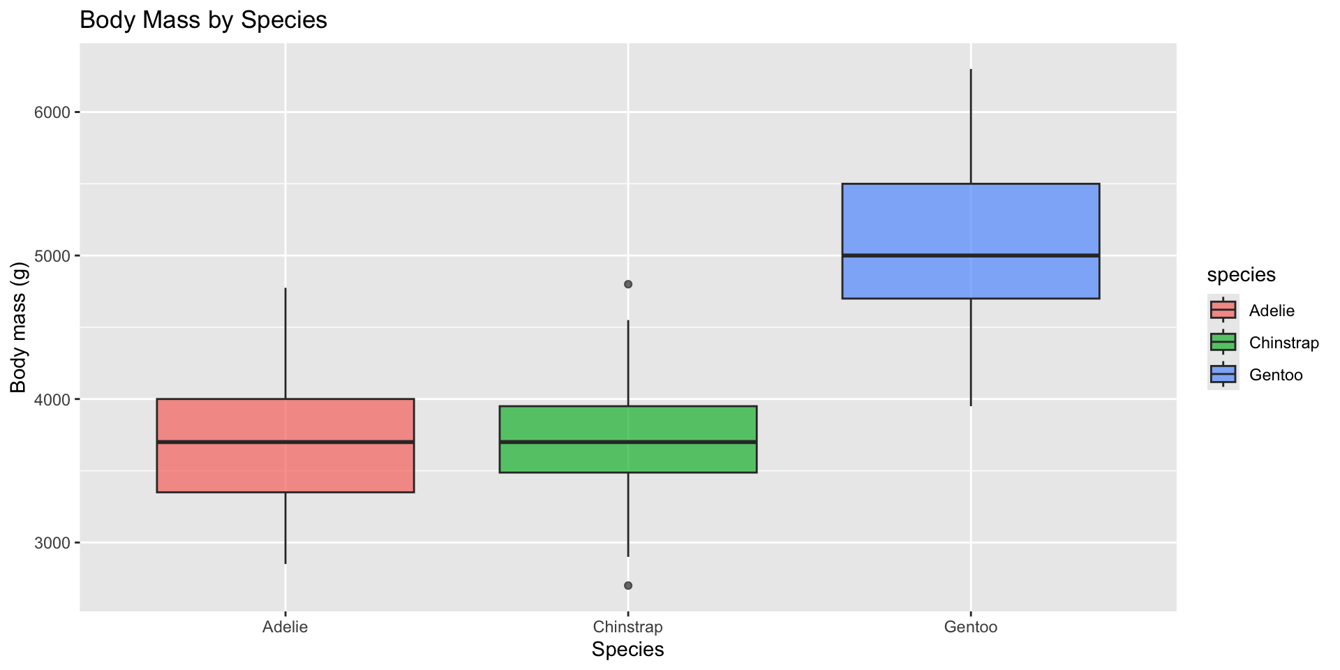
Boxplot — spread across groups
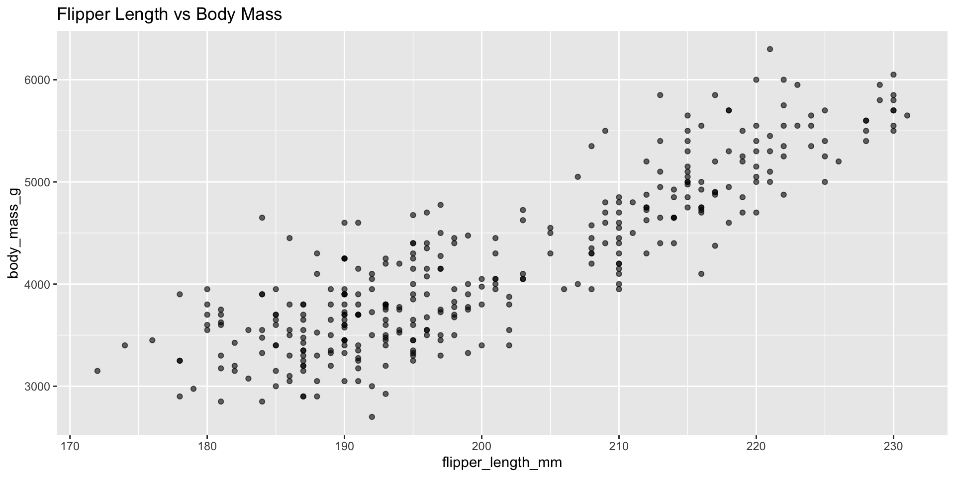
Scatterplot
Correlation (descriptive, not yet a test)
cor() gives a single number (-1 to 1) summarising the strength and direction of a linear relationship.
From Description to Inference
What a p-value actually means
- Null hypothesis (H₀): no real difference/relationship exists in the population; anything we see in our sample is due to chance
- A p-value is the probability of seeing a difference this large, if H₀ were true
- Small p-value (conventionally < 0.05) → the data would be unusual under H₀ → we reject H₀
What a p-value is not:
It is not the probability that H₀ is true, and it is not the probability your result is “important.” A tiny p-value can come from a trivial effect if the sample is large enough — always report the effect size alongside it.
The general workflow for every test
- State H₀ (no difference/relationship) and H₁ (there is one)
- Check the test’s assumptions
- Run the test in R
- Read the p-value and the effect size / confidence interval
- Write one sentence of plain-language interpretation
Comparing Two Groups
Independent-samples t-test
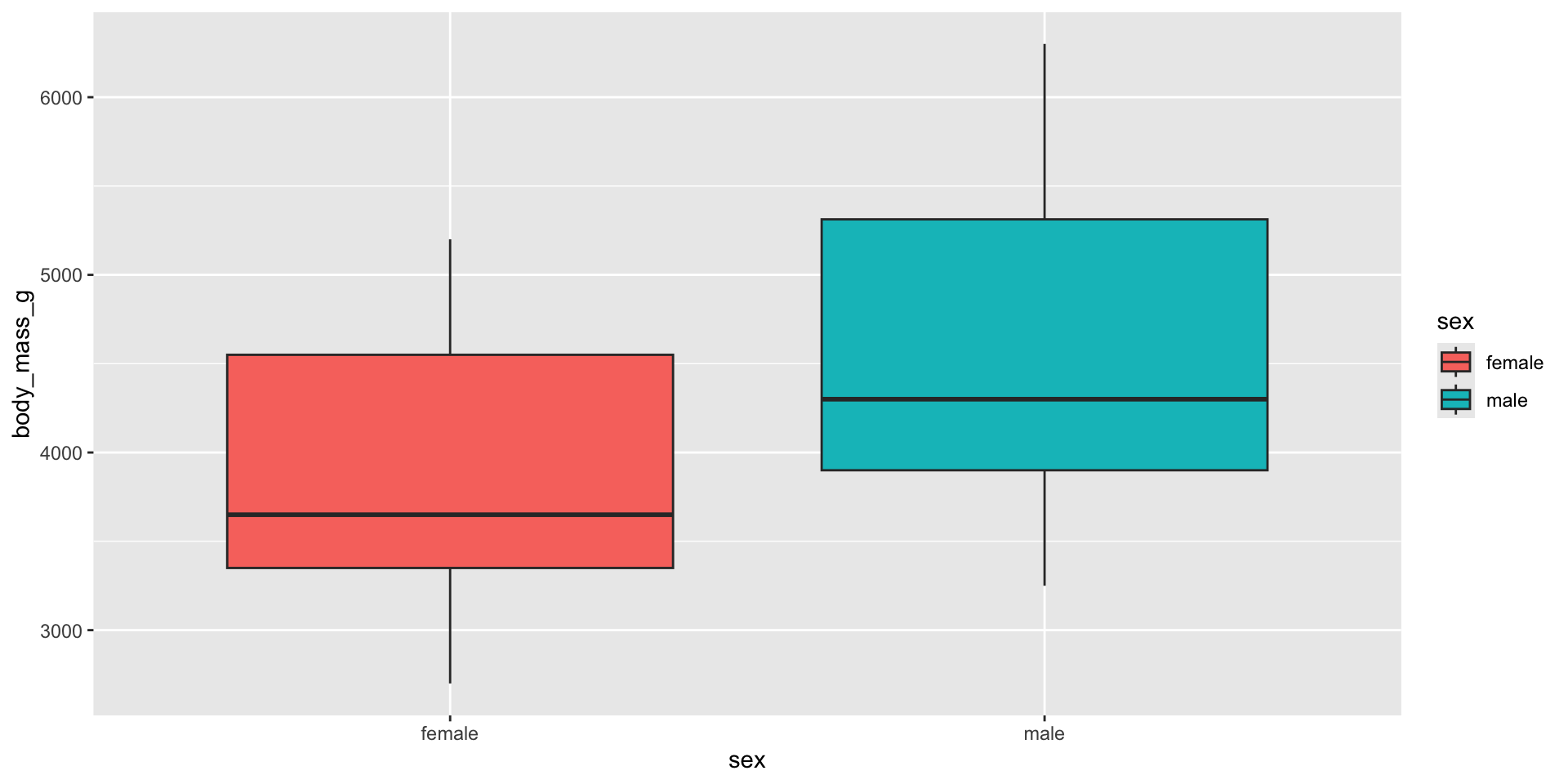
Question: Does body mass differ between male and female penguins?
Running the t-test
    Welch Two Sample t-test

data:  body_mass_g by sex
t = -8.5545, df = 323.9, p-value = 4.794e-16
alternative hypothesis: true difference in means between group female and group male is not equal to 0
95 percent confidence interval:
 -840.5783 -526.2453
sample estimates:
mean in group female   mean in group male
            3862.273             4545.685
Reading the output:
t= test statistic,df= degrees of freedomp-value— here, extremely small → strong evidence of a real difference95% confidence interval — the likely range for the true difference in means
Reports means for each group at the bottom
“Male penguins have significantly more weight than female penguins (p < .001)”
Your Turn
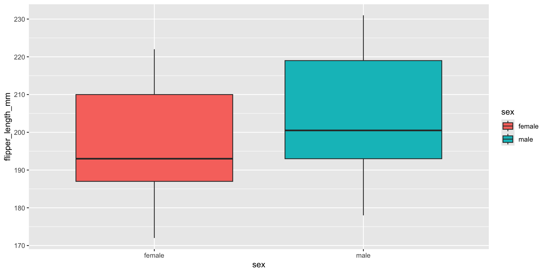
Test whether flipper_length_mm differs by sex.
- Boxplot first
- Run
t.test() - Write one sentence interpreting the result
Answer
Answer
    Welch Two Sample t-test

data:  flipper_length_mm by sex
t = -4.8079, df = 325.28, p-value = 2.336e-06
alternative hypothesis: true difference in means between group female and group male is not equal to 0
95 percent confidence interval:
 -10.064811  -4.219821
sample estimates:
mean in group female   mean in group male
            197.3636             204.5060
“Male penguins have significantly longer flippers than female penguins (p < .001).”
Comparing Three or More Groups
One-way ANOVA
Question: does body mass differ across the three species?
             Df    Sum Sq  Mean Sq F value Pr(>F)
species       2 145190219 72595110   341.9 <2e-16 ***
Residuals   330  70069447   212332
---
Signif. codes:  0 '***' 0.001 '**' 0.01 '*' 0.05 '.' 0.1 ' ' 1
ANOVA tests whether at least one group differs from the others — it does not tell you which pair(s) differ. The significant Pr(>F) here says species matters, but we need a follow-up test to know which species differ from which.
Post-hoc test: Tukey HSD
  Tukey multiple comparisons of means
    95% family-wise confidence level

Fit: aov(formula = body_mass_g ~ species, data = penguins)

$species
                       diff       lwr       upr    p adj
Chinstrap-Adelie   26.92385 -132.3528  186.2005 0.916431
Gentoo-Adelie    1386.27259 1252.2897 1520.2554 0.000000
Gentoo-Chinstrap 1359.34874 1194.4304 1524.2671 0.000000
Every pairwise comparison, with an adjusted p-value that corrects for multiple testing. Reading the output: adelie-Gentoo, Adelie-Chinstrap, Chinstrap-Gentoo — check the p adj column for each pair.
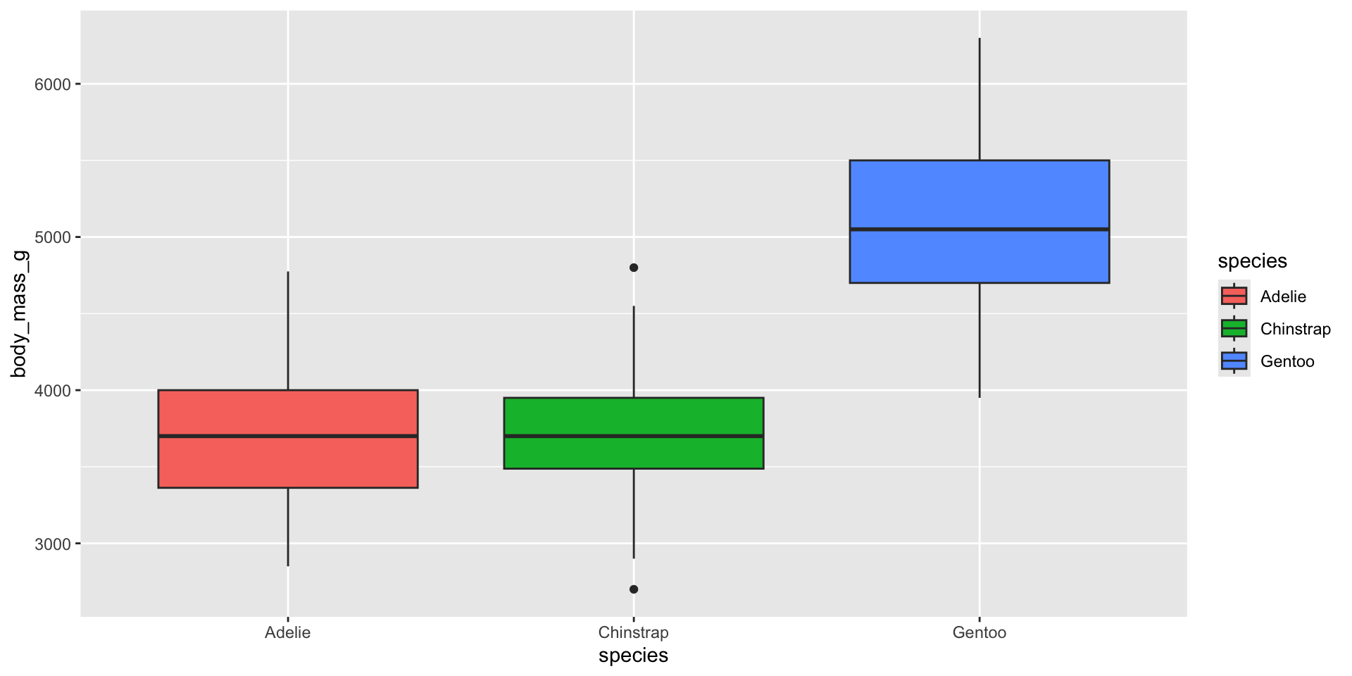
Checking ANOVA assumptions visually
Your Turn
- Run an ANOVA testing whether
flipper_length_mmdiffers byspecies - Run
TukeyHSD()on it - Which species pairs differ significantly?
Answer
             Df Sum Sq Mean Sq F value Pr(>F)
species       2  50526   25263   567.4 <2e-16 ***
Residuals   330  14693      45
---
Signif. codes: 0 '***' 0.001 '**' 0.01 '*' 0.05 '.' 0.1 ' ' 1 Tukey multiple comparisons of means
95% family-wise confidence level
Fit: aov(formula = flipper_length_mm ~ species, data = penguins)
$species
diff lwr upr p adj
Chinstrap-Adelie 5.72079 3.414364 8.027215 0
Gentoo-Adelie 27.13255 25.192399 29.072709 0
Gentoo-Chinstrap 21.41176 19.023644 23.799885 0All three pairwise comparisons are significant — every species differs from every other in flipper length.
Testing Relationships
Correlation test
    Pearson's product-moment correlation

data:  penguins$bill_length_mm and penguins$flipper_length_mm
t = 15.691, df = 331, p-value < 2.2e-16
alternative hypothesis: true correlation is not equal to 0
95 percent confidence interval:
 0.5868092 0.7106869
sample estimates:
      cor
0.6530956
plain cor() — now we get a p-value and confidence interval alongside the correlation coefficient (cor in the output), telling us whether this relationship is distinguishable from zero.
Chi-square test of independence
Question: is species associated with island?
            Biscoe Dream Torgersen
  Adelie        44    55        47
  Chinstrap      0    68         0
  Gentoo       119     0         0
    Pearson's Chi-squared test

data:  tbl
X-squared = 284.59, df = 4, p-value < 2.2e-16
Chi-square tests whether two categorical variables are independent. Here, the tiny p-value confirms — species and island are strongly associated
Your Turn
- Test the correlation between
bill_depth_mmandbody_mass_gwithcor.test() - Build a table of
speciesbysexand run a chi-square test — are they associated?
Answer
    Pearson's product-moment correlation

data:  penguins$bill_depth_mm and penguins$body_mass_g
t = -9.741, df = 331, p-value < 2.2e-16
alternative hypothesis: true correlation is not equal to 0
95 percent confidence interval:
 -0.5515130 -0.3840214
sample estimates:
       cor
-0.4720157
            female male
  Adelie        73   73
  Chinstrap     34   34
  Gentoo        58   61
    Pearson's Chi-squared test

data:  tbl2
X-squared = 0.048607, df = 2, p-value = 0.976
Species and sex are not significantly associated (roughly equal male/female split within each species) — a good example of a non-significant, and equally informative, result.
Choosing the Right Test
A quick decision guide
| Question | Variable types | Test |
|---|---|---|
| Do 2 groups differ? | 1 numeric + 1 categorical (2 levels) | t.test() |
| Do 3+ groups differ? | 1 numeric + 1 categorical (3+ levels) | aov() + TukeyHSD() |
| Are two numeric variables related? | 2 numeric | cor.test() |
| Are two categorical variables associated? | 2 categorical | chisq.test() |
Simple Linear Regression
From correlation to regression
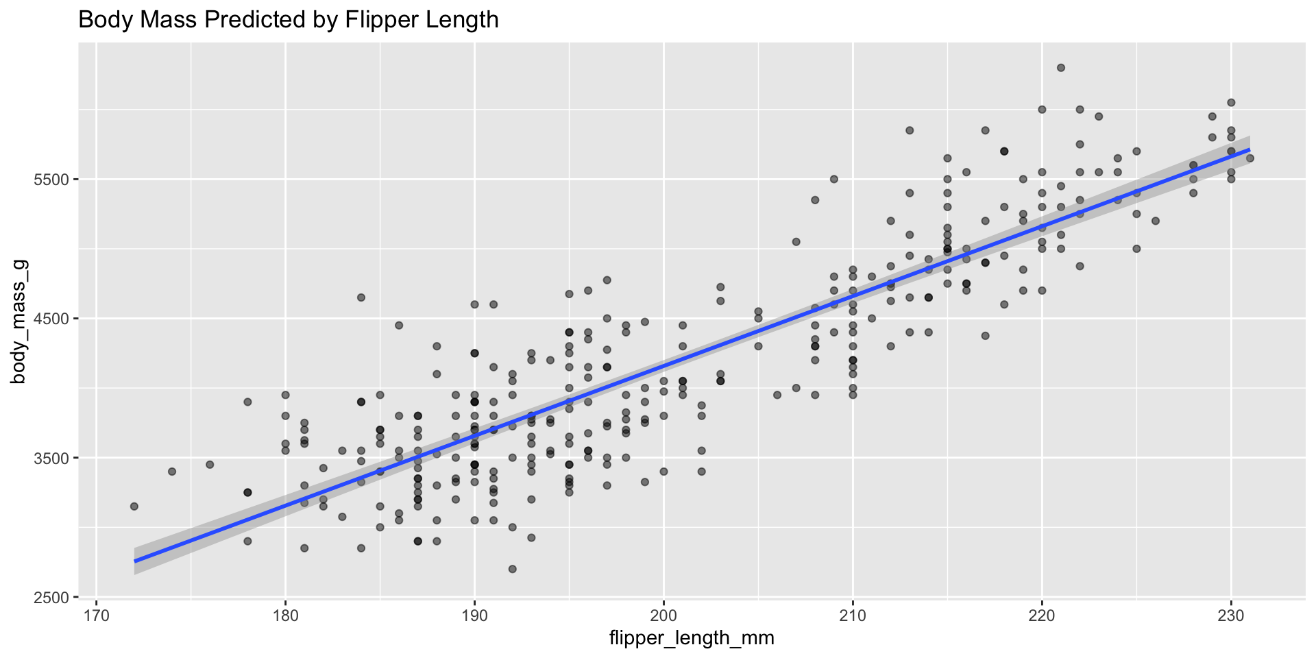
cor.test()told us whetherflipper_length_mmandbody_mass_gare related, and how strongly- Regression goes further: it gives us an equation to predict one from the other
Call:
lm(formula = body_mass_g ~ flipper_length_mm, data = penguins)

Residuals:
     Min       1Q   Median       3Q      Max
-1057.33  -259.79   -12.24   242.97  1293.89

Coefficients:
                  Estimate Std. Error t value Pr(>|t|)
(Intercept)       -5872.09     310.29  -18.93   <2e-16 ***
flipper_length_mm    50.15       1.54   32.56   <2e-16 ***
---
Signif. codes:  0 '***' 0.001 '**' 0.01 '*' 0.05 '.' 0.1 ' ' 1

Residual standard error: 393.3 on 331 degrees of freedom
Multiple R-squared:  0.7621,    Adjusted R-squared:  0.7614
F-statistic:  1060 on 1 and 331 DF,  p-value: < 2.2e-16
Reading the output
- Intercept: predicted
body_mass_gwhenflipper_length_mm= 0 (often not meaningful on its own) - Slope (
flipper_length_mmcoefficient): for every 1mm increase in flipper length, body mass increases by this many grams - p-value (per coefficient): is this slope distinguishable from zero?
- R-squared: proportion of variance in
body_mass_gexplained byflipper_length_mm(0 to 1)
Visualising the fitted line
Your Turn 1
- Fit
lm(bill_length_mm ~ bill_depth_mm, data = penguins) - What is the slope? Is it significant?
- What is the R²? How much variance is explained?
Answer
Call:
lm(formula = bill_length_mm ~ bill_depth_mm, data = penguins)

Residuals:
     Min       1Q   Median       3Q      Max
-12.9498  -3.9530  -0.3657   3.7327  15.5025

Coefficients:
              Estimate Std. Error t value Pr(>|t|)
(Intercept)    54.8909     2.5673  21.380  < 2e-16 ***
bill_depth_mm  -0.6349     0.1486  -4.273 2.53e-05 ***
---
Signif. codes:  0 '***' 0.001 '**' 0.01 '*' 0.05 '.' 0.1 ' ' 1

Residual standard error: 5.332 on 331 degrees of freedom
Multiple R-squared:  0.05227,   Adjusted R-squared:  0.04941
F-statistic: 18.26 on 1 and 331 DF,  p-value: 2.528e-05
The slope is negative and significant here
Thank you!
Module 4 complete 🎉
SARA Institute of Data Science - 3rd SARA Summer School 22-26 July 2026 “R for Researchers”
Course Slides website: https://sara-course-r4b.netlify.app/