SARA | The Non-Profit – Data Visualisation

Data Visualization

“The simple graph has brough more information to the data analyst’s mind than any other device.” - John Tukey

Climate Spiral

The R Graph Gallery

Computational Art

Grammar of Graphics

“ggplot2 implements grammar of graphics, a coherent system for describing and building graphs”

Set-up

```{r}
#| label: set-up-data-viz
library(palmerpenguins) # to access peguins data

# to access ggplot2 package
library(tidyverse)
```

Know your Data

glimpse(penguins)

Rows: 344
Columns: 8
$ species           <fct> Adelie, Adelie, Adelie, Adelie, Adelie, Adelie, Adel…
$ island            <fct> Torgersen, Torgersen, Torgersen, Torgersen, Torgerse…
$ bill_length_mm    <dbl> 39.1, 39.5, 40.3, NA, 36.7, 39.3, 38.9, 39.2, 34.1, …
$ bill_depth_mm     <dbl> 18.7, 17.4, 18.0, NA, 19.3, 20.6, 17.8, 19.6, 18.1, …
$ flipper_length_mm <int> 181, 186, 195, NA, 193, 190, 181, 195, 193, 190, 186…
$ body_mass_g       <int> 3750, 3800, 3250, NA, 3450, 3650, 3625, 4675, 3475, …
$ sex               <fct> male, female, female, NA, female, male, female, male…
$ year              <int> 2007, 2007, 2007, 2007, 2007, 2007, 2007, 2007, 2007…

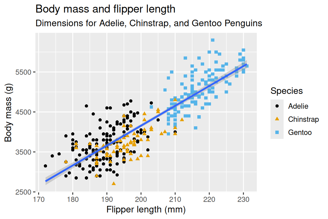
Ultimate Goal

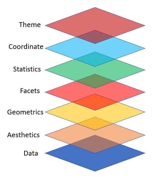
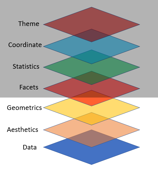
ggplot2 Layers

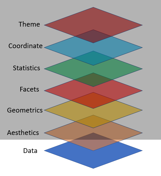
ggplot(data = penguins)

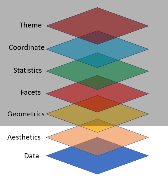
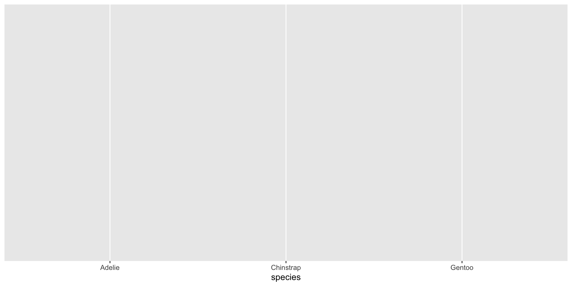
Map Variables Aesthetics

Task
Code
Output

ggplot(data = penguins, 
        mapping = aes(x = species))

Add Geometric Shapes

Task
Code
Output

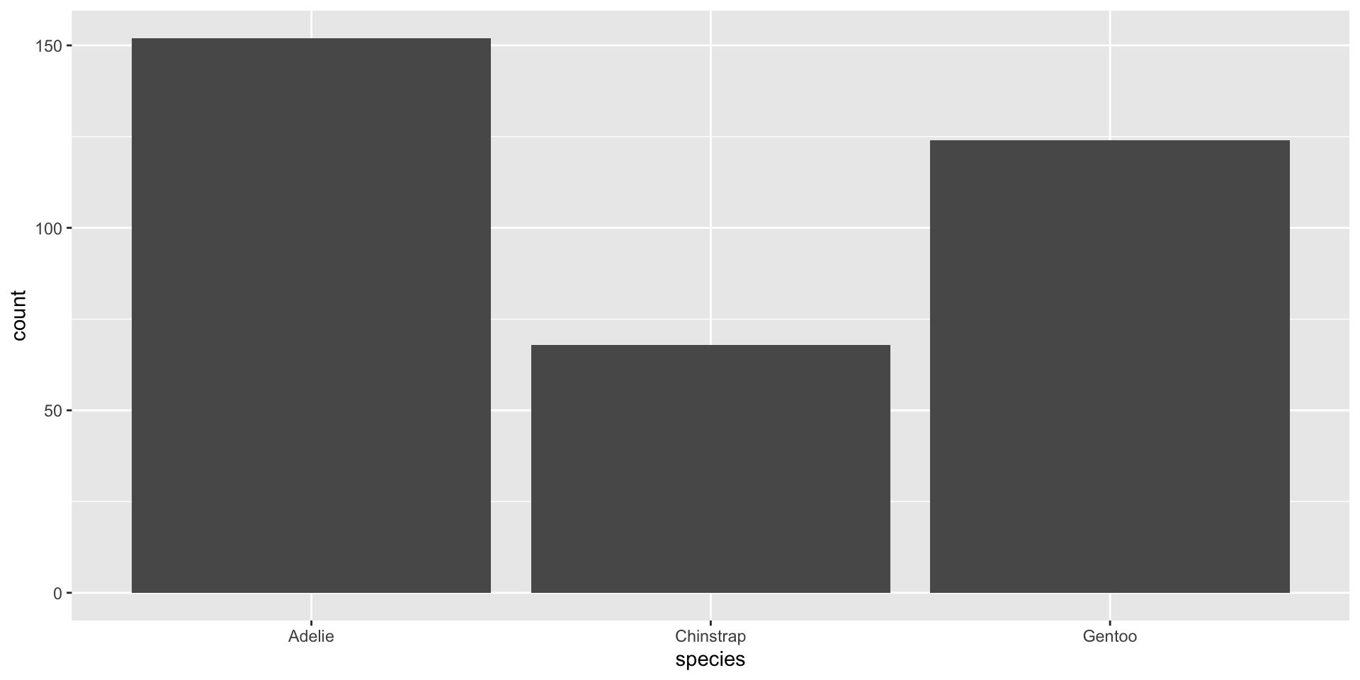
ggplot(data = penguins, 
        mapping = aes(x = species)) +
          geom_bar()

Caution

Common beginner mistake: putting + at the start of a new line instead of the end of the previous line. R needs the + at the end to know more is coming!

Key Components are:

Data - which data frame?
Aesthetics (aes) - which columns map to x, y, colour, size…?
Geometry (geom) - what type of plot? points, bars, lines…

🧠 YOUR TURN

Task
Answer

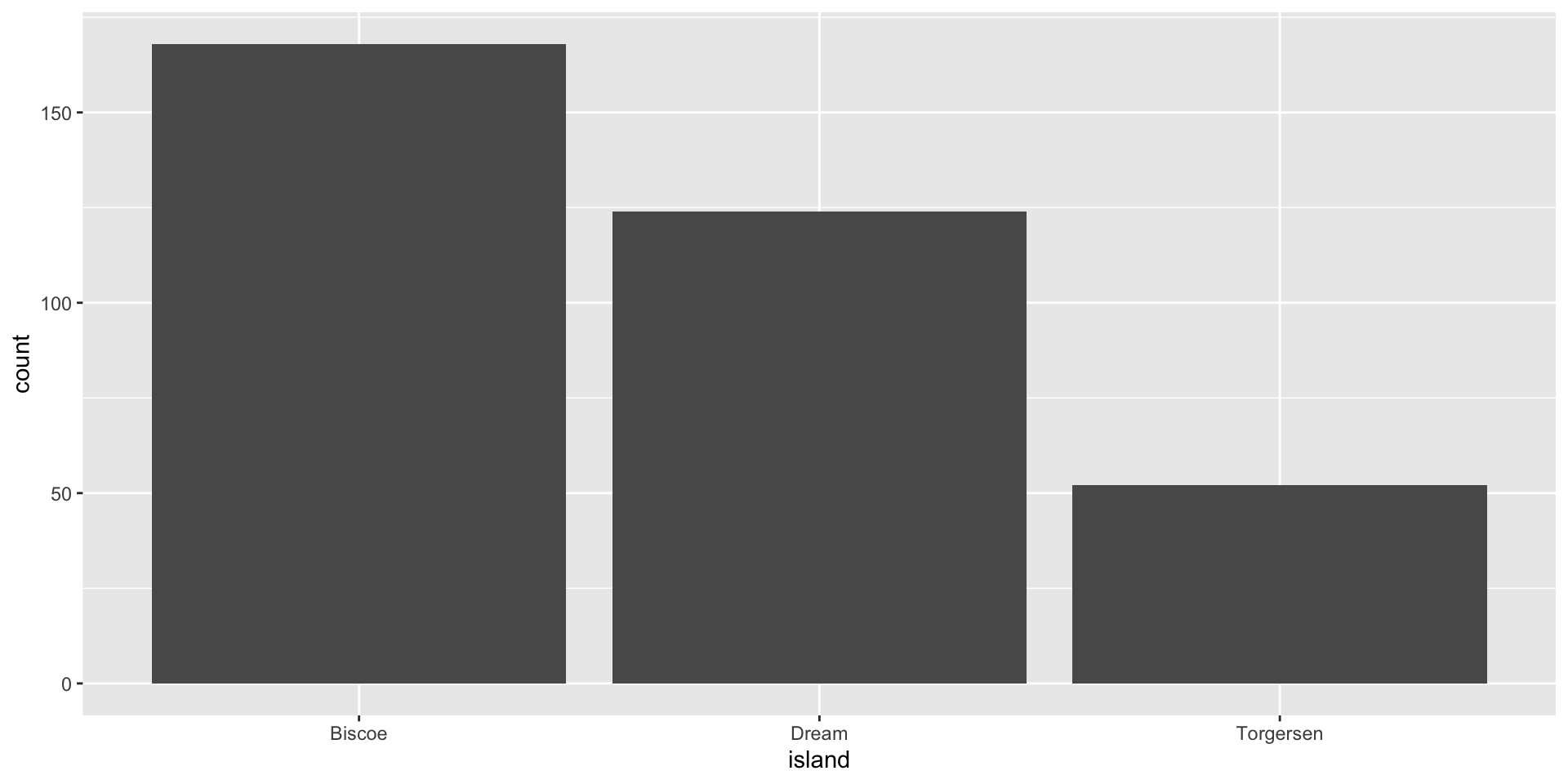
ggplot(data = penguins, 
        mapping = aes(x = island)) +
        geom_bar()

“Fill” Color

Task
Code
Output

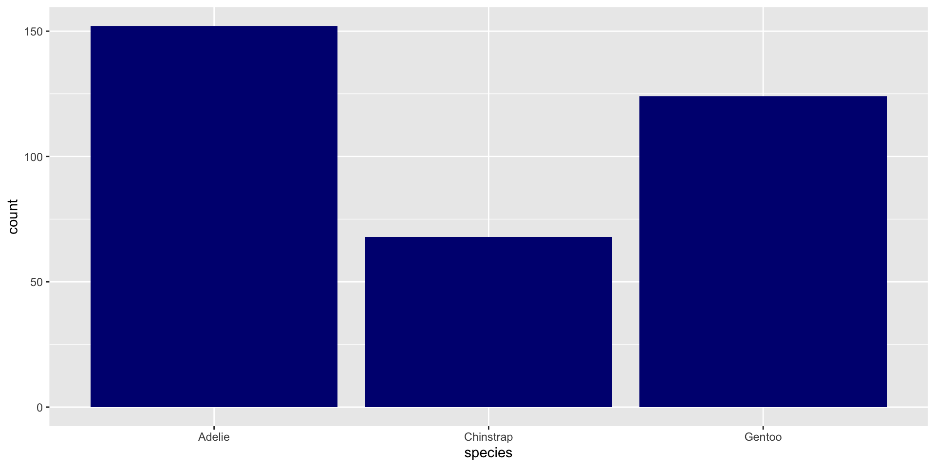
ggplot(data = penguins, 
      mapping = aes(x = species)) +
        geom_bar(fill = "navy")

“Fill” Colors

Task
Code
Output

ggplot(data = penguins, 
      mapping = aes(x = species)) +
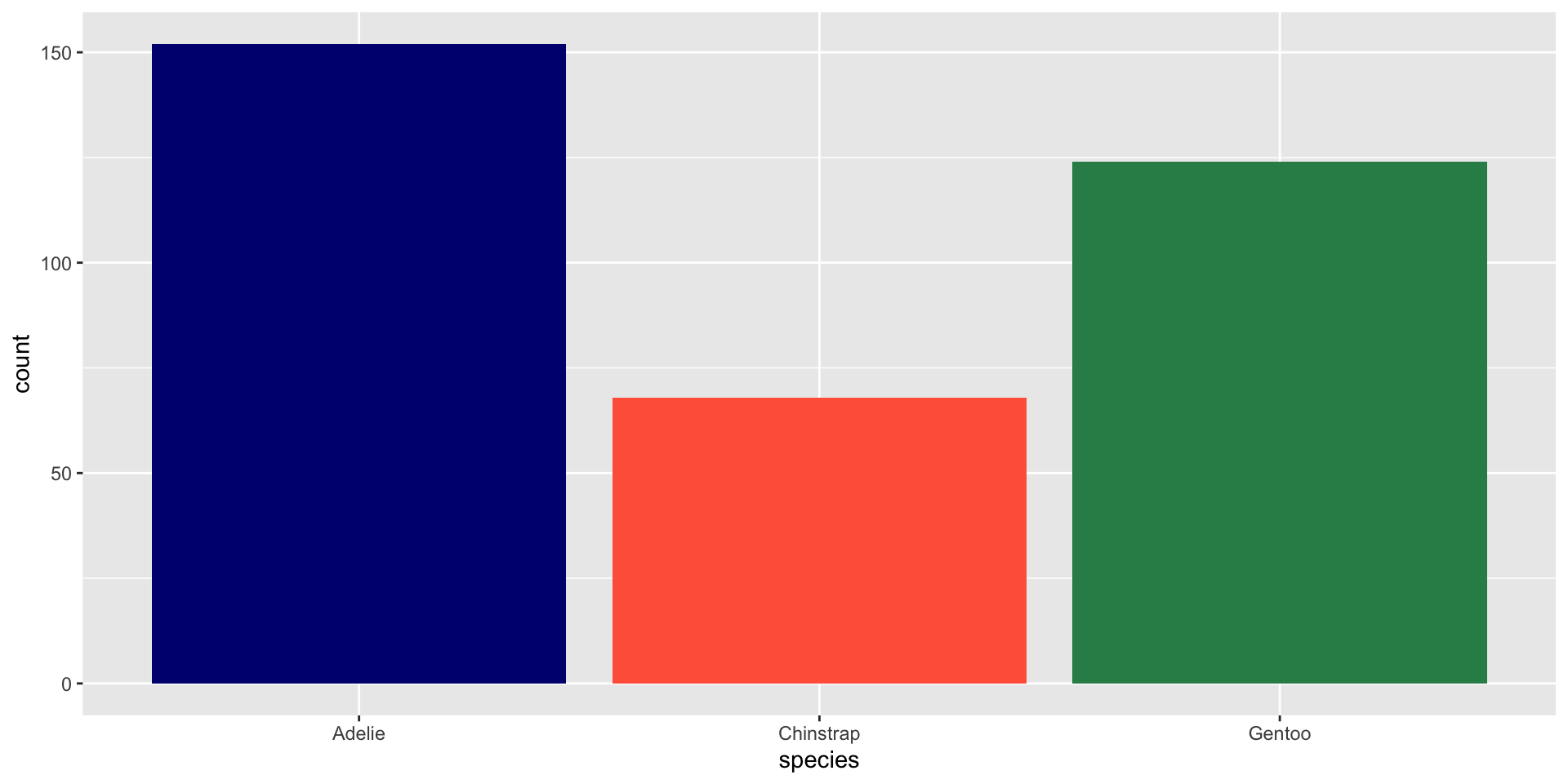
        geom_bar(fill = c("navy", "tomato", "seagreen"))

“Fill” Colors vs “Color” Colors

Task
Code
Output

ggplot(data = penguins,
      mapping = aes(x = species)) +
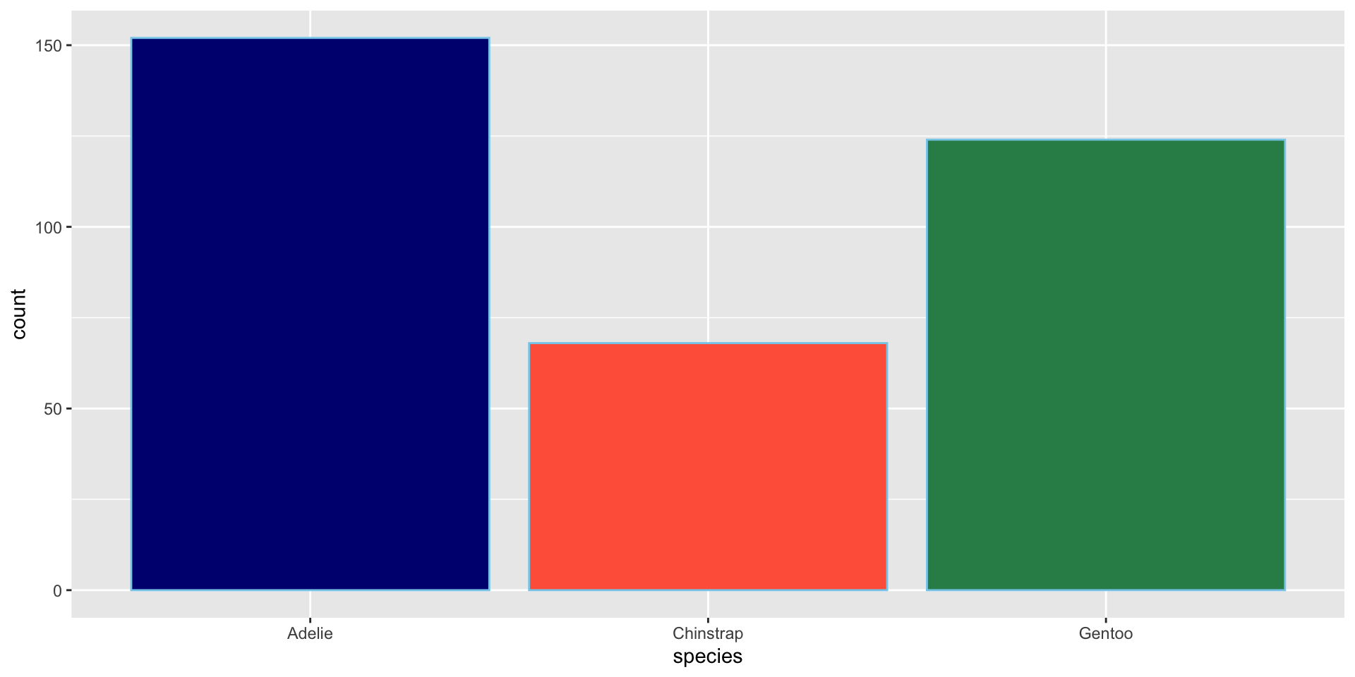
        geom_bar(fill = c("navy", "tomato", "seagreen"),
        color = "skyblue")

📝 YOUR TURN

Task
Answer

ggplot(data = penguins,
       mapping = aes(x = island)) +
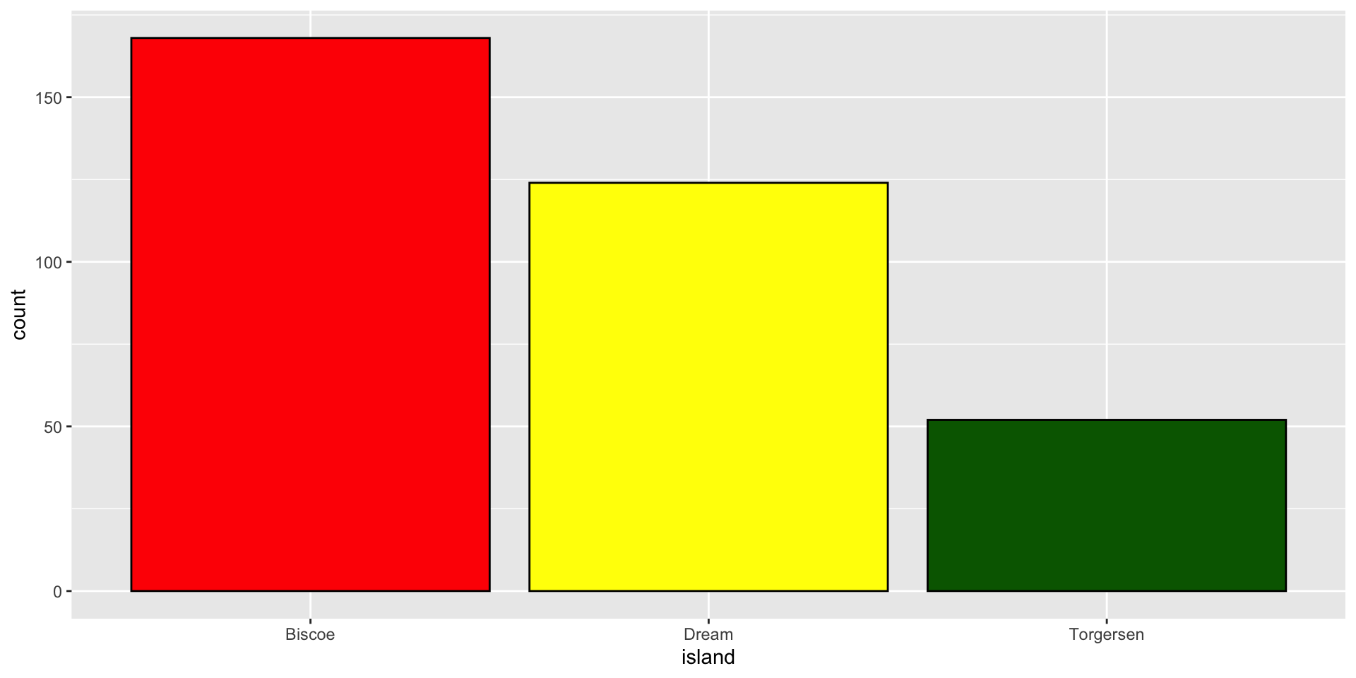
  geom_bar(fill = c("red", "yellow", "darkgreen"),
           color = "black")

Plot A Continuous Variable

Task
Code
Output

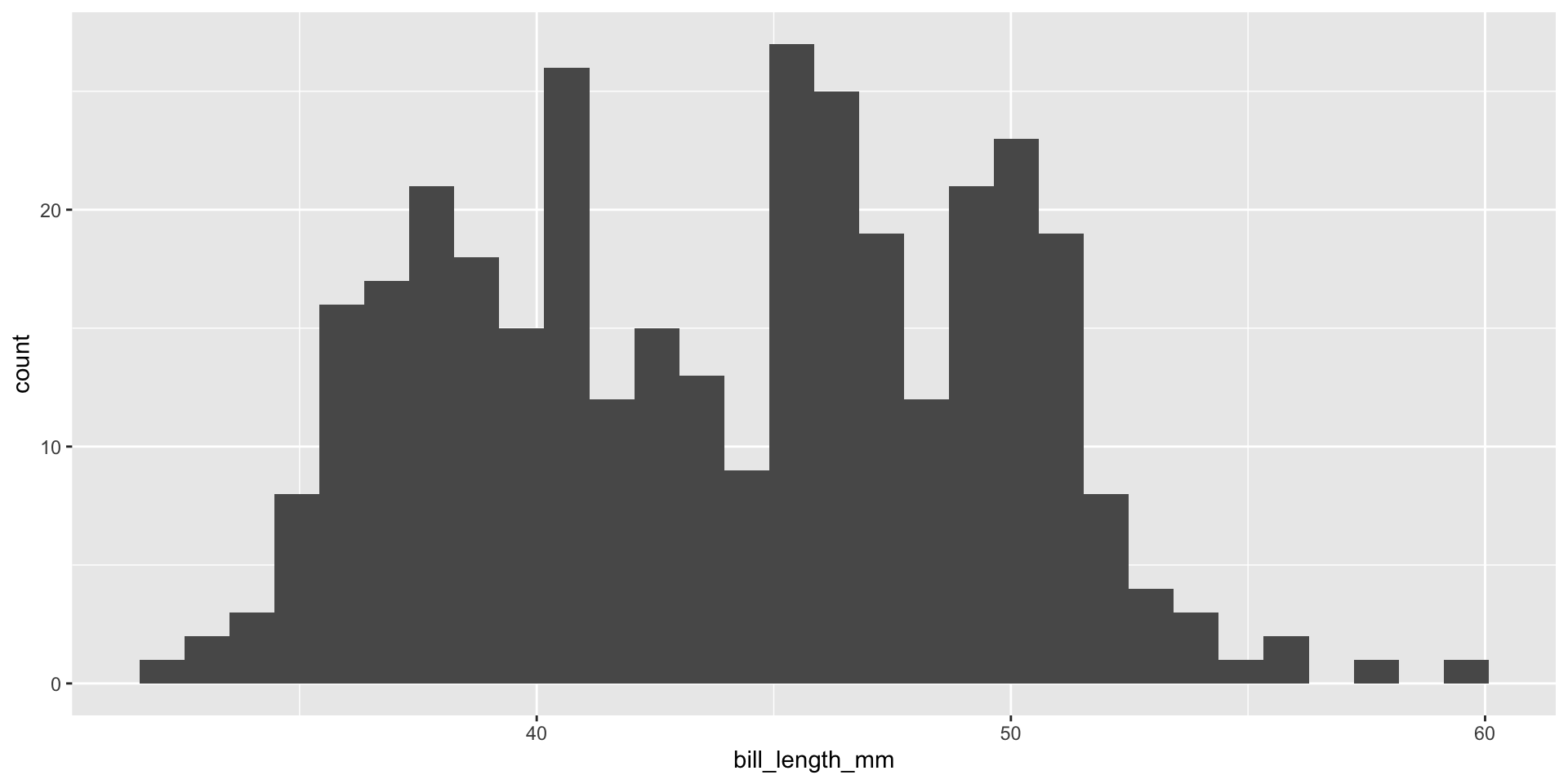
# bill_length_mm is dbl type variable/column

ggplot(data = penguins,
       mapping = aes(x = bill_length_mm)) +
  geom_histogram()

🧠 YOUR TURN

Task
Answer

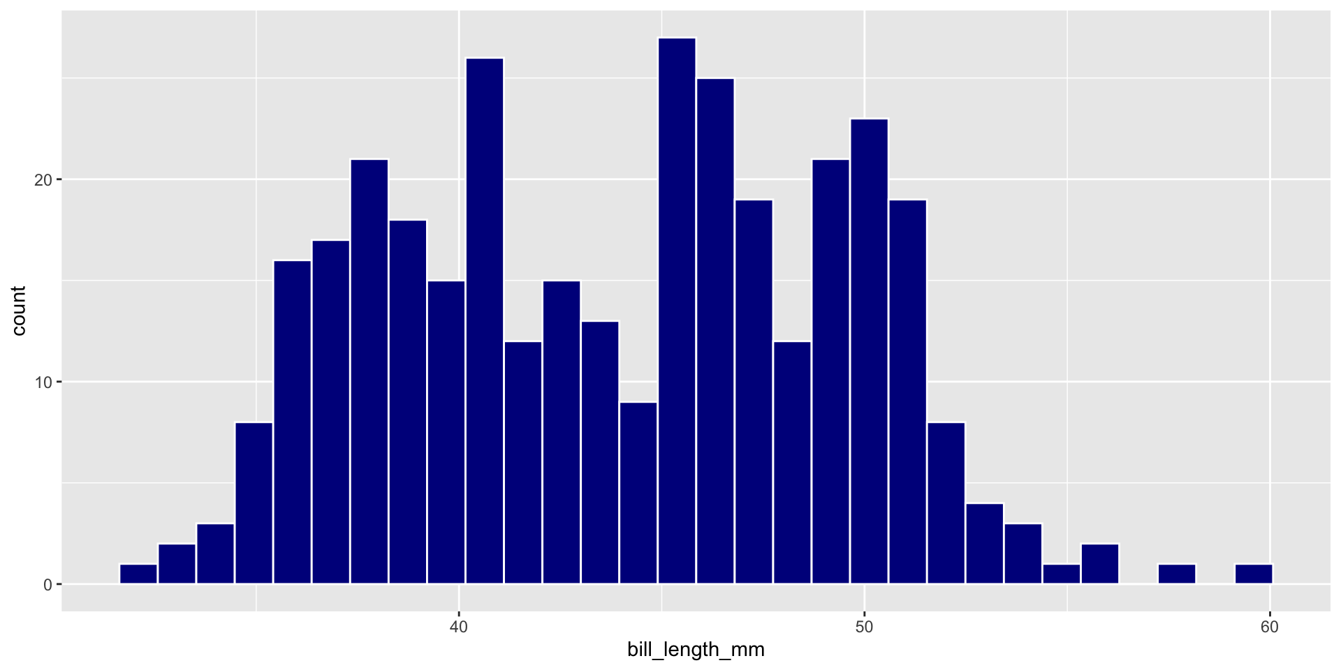
ggplot(data = penguins,
       mapping = aes(x = bill_length_mm)) +
  geom_histogram(fill = "darkblue",
                 color = "white")

Two Continuous Variables

Task
Code
Output

ggplot(data = penguins,
       mapping = aes(x = bill_length_mm, y = bill_depth_mm)) +
  geom_point()

Geom Size

Task
Code
Output

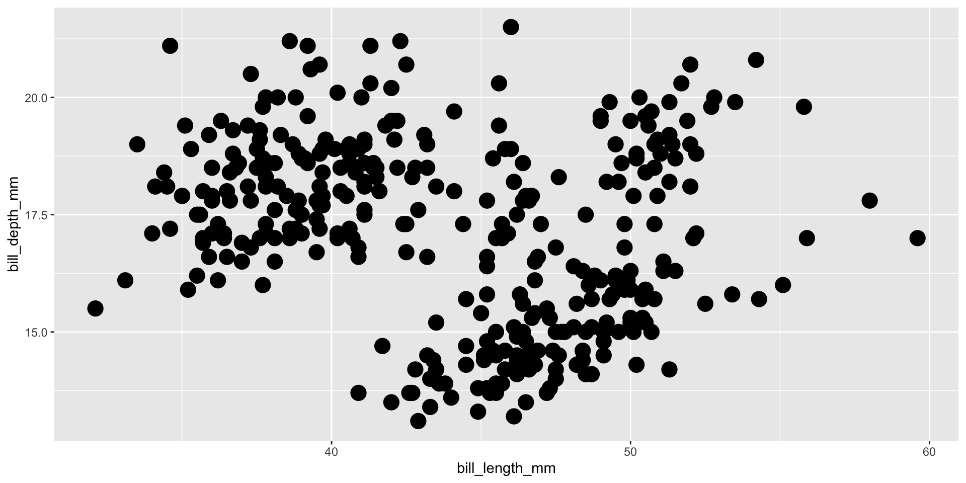
ggplot(data = penguins,
       mapping = aes(x = bill_length_mm, y = bill_depth_mm)) +
  geom_point(size = 5)

Geom Shape

Task
Code
Output

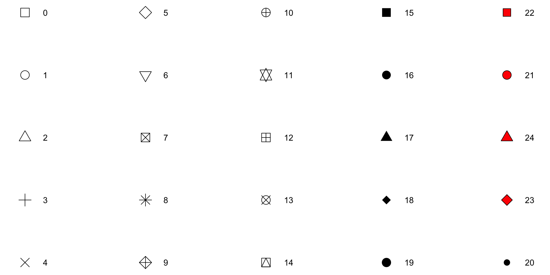
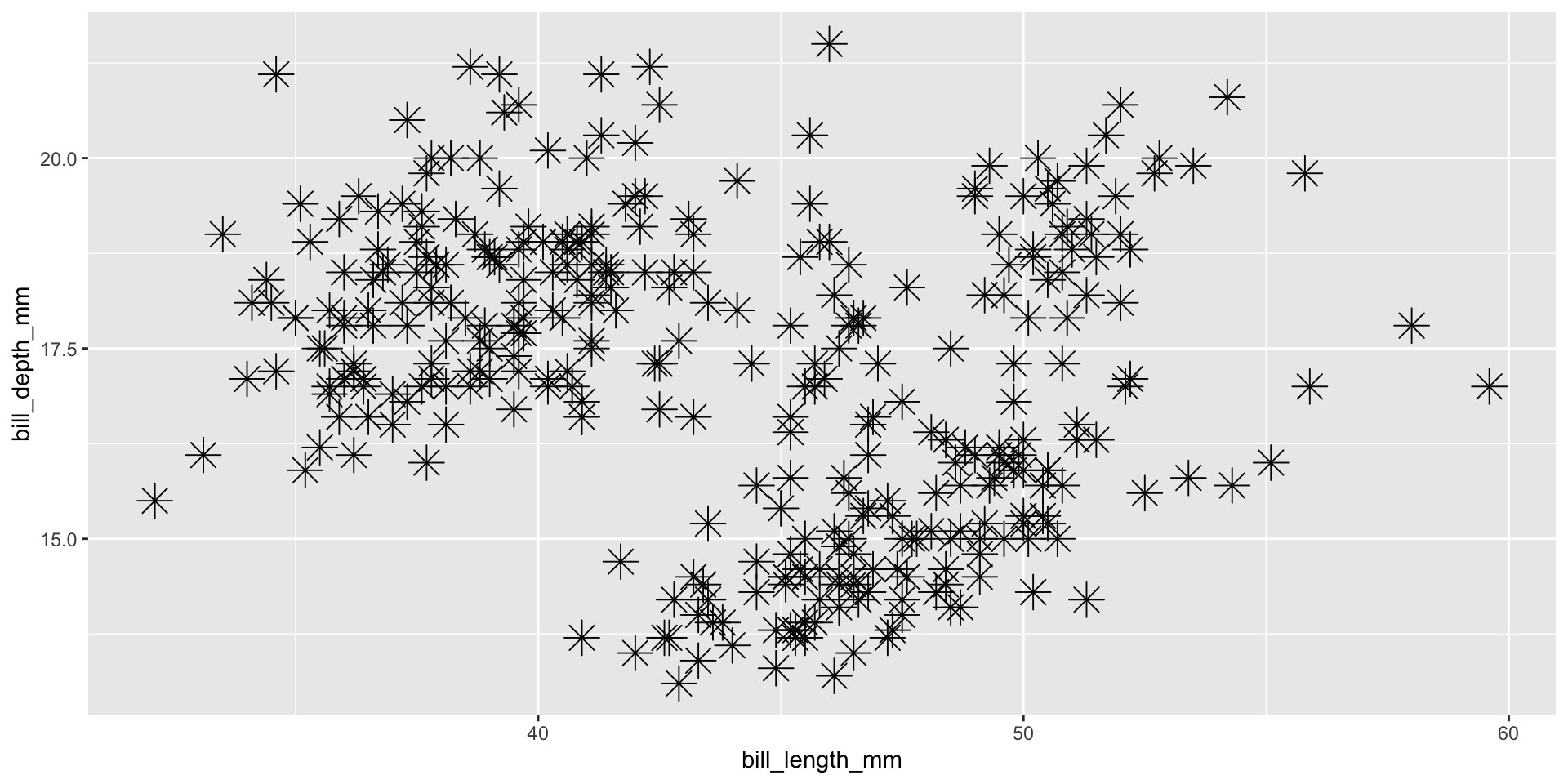
ggplot(data = penguins,
       mapping = aes(x = bill_length_mm, y = bill_depth_mm)) +
  geom_point(size = 5,
             shape = 8)

📝 YOUR TURN

Task
Answer

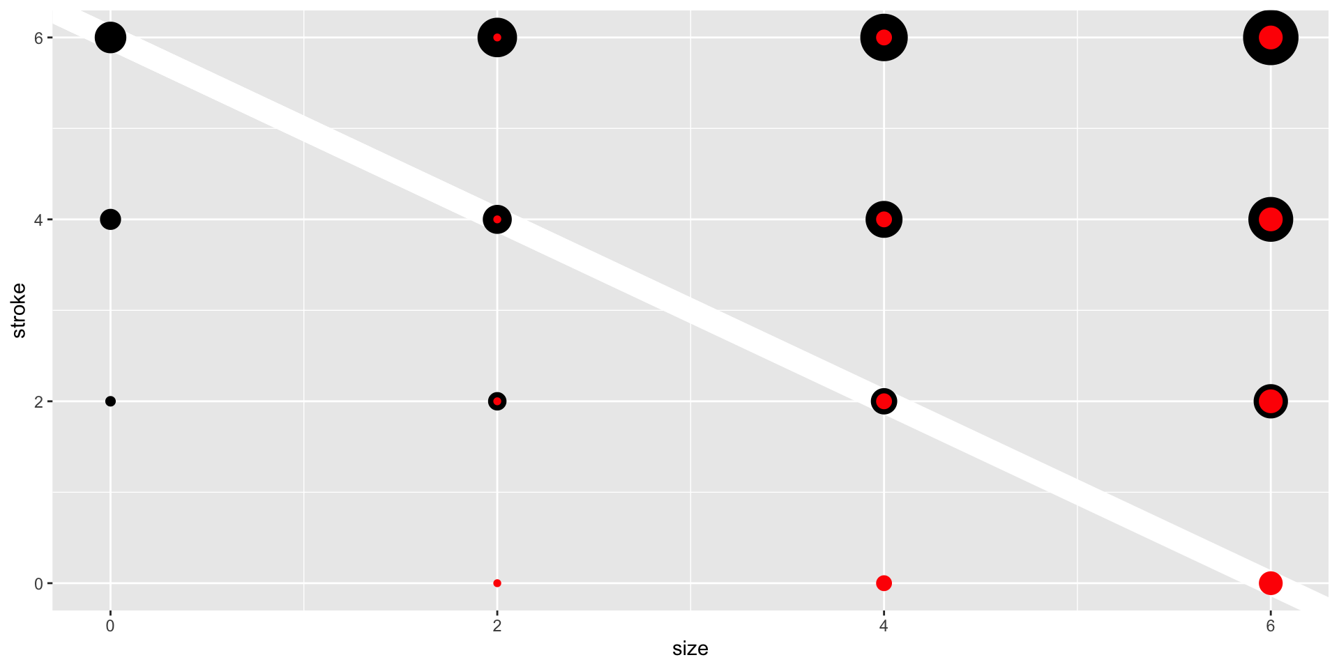
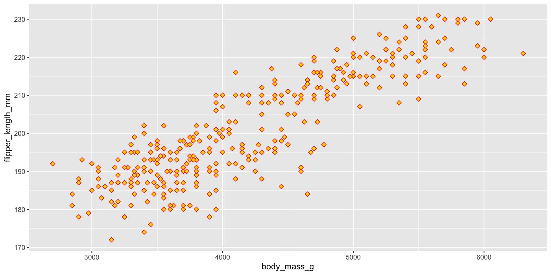
ggplot(data = penguins,
       mapping = aes(x = body_mass_g, y = flipper_length_mm)) +
  geom_point(size = 2, shape = 23, color = "red", fill = "gold")

Plot A Factor & Factor

Task
Code
Output

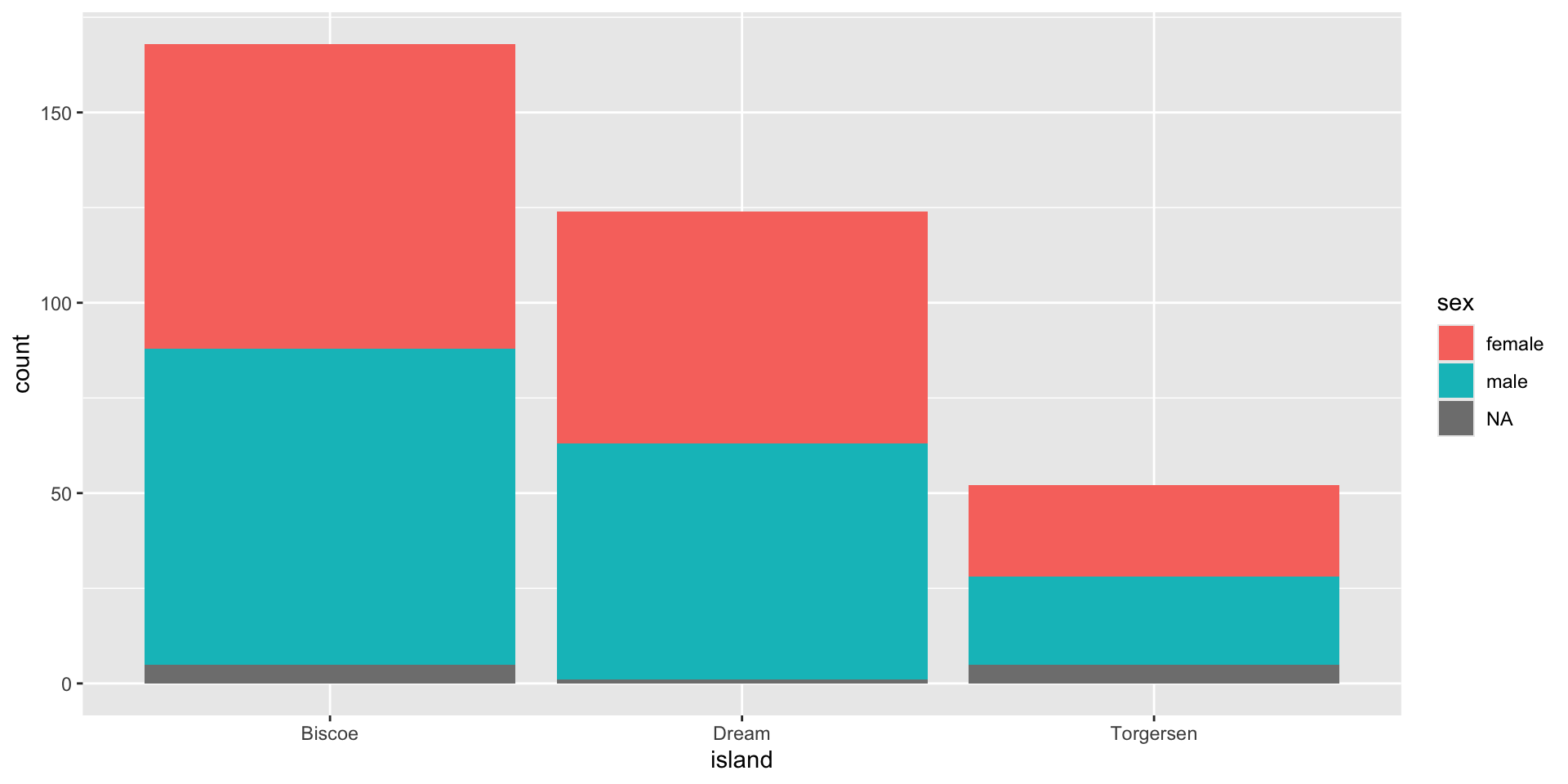
Sometimes, we want to differentiate values of a factor/category variable on the basis of another factor/category variable.

ggplot(data = penguins,
       mapping = aes(x = island)) +
  geom_bar(aes(fill = sex))

Plot A Factor & Continuous

Task
Code
Output

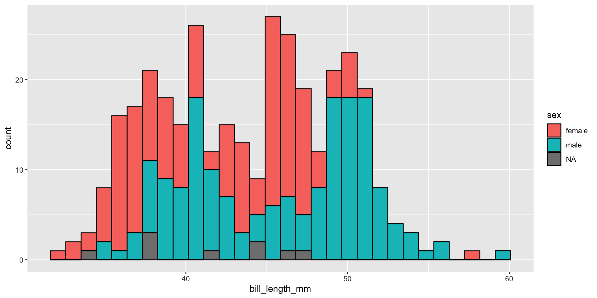
Sometimes, we want to differentiate values from a continuous variable on the basis of factor/category variables.

ggplot(data = penguins,
       mapping = aes(x = bill_length_mm)) +
  geom_histogram(aes(fill = sex), color = "black")

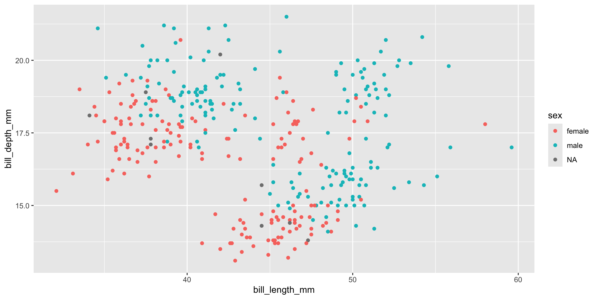
A Factor & Two Cont. Variables

Task
Code
Output

ggplot(data = penguins,
       mapping = aes(x = bill_length_mm, y = bill_depth_mm)) +
  geom_point(aes(color = sex))

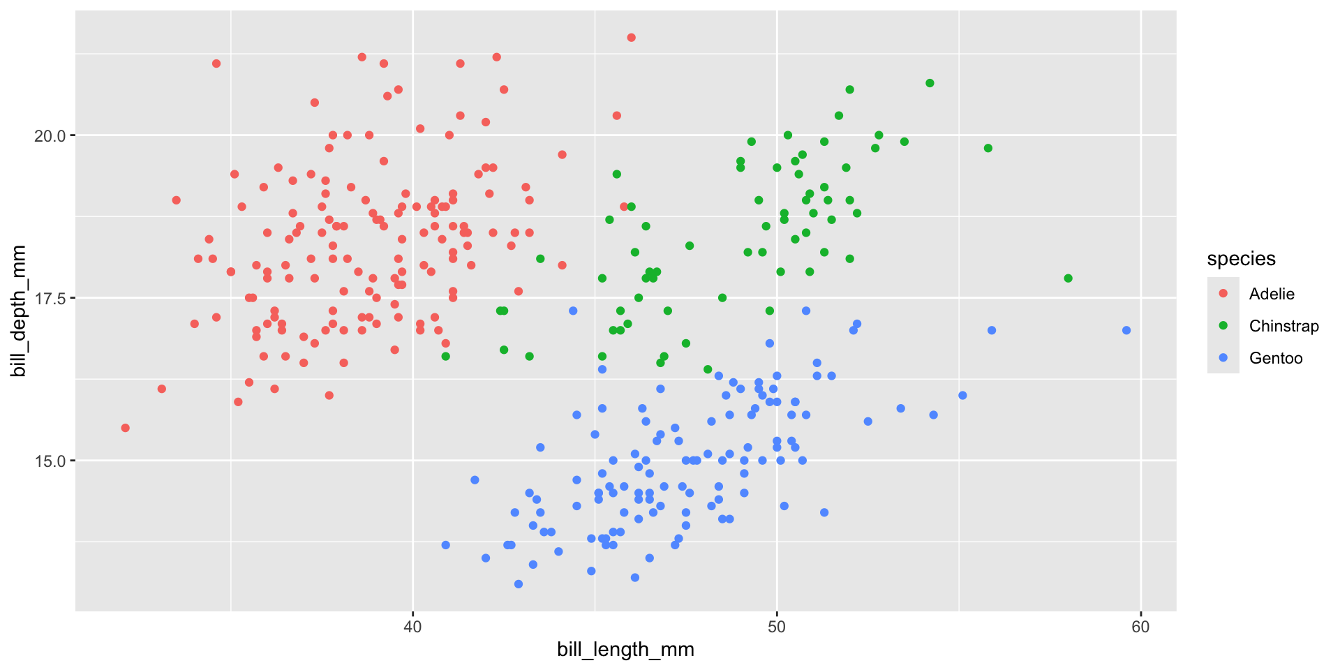
A Factor & Two Cont. Variables

Task
Code
Output

ggplot(data = penguins,
       mapping = aes(x = bill_length_mm, y = bill_depth_mm)) +
  geom_point(aes(color = species))

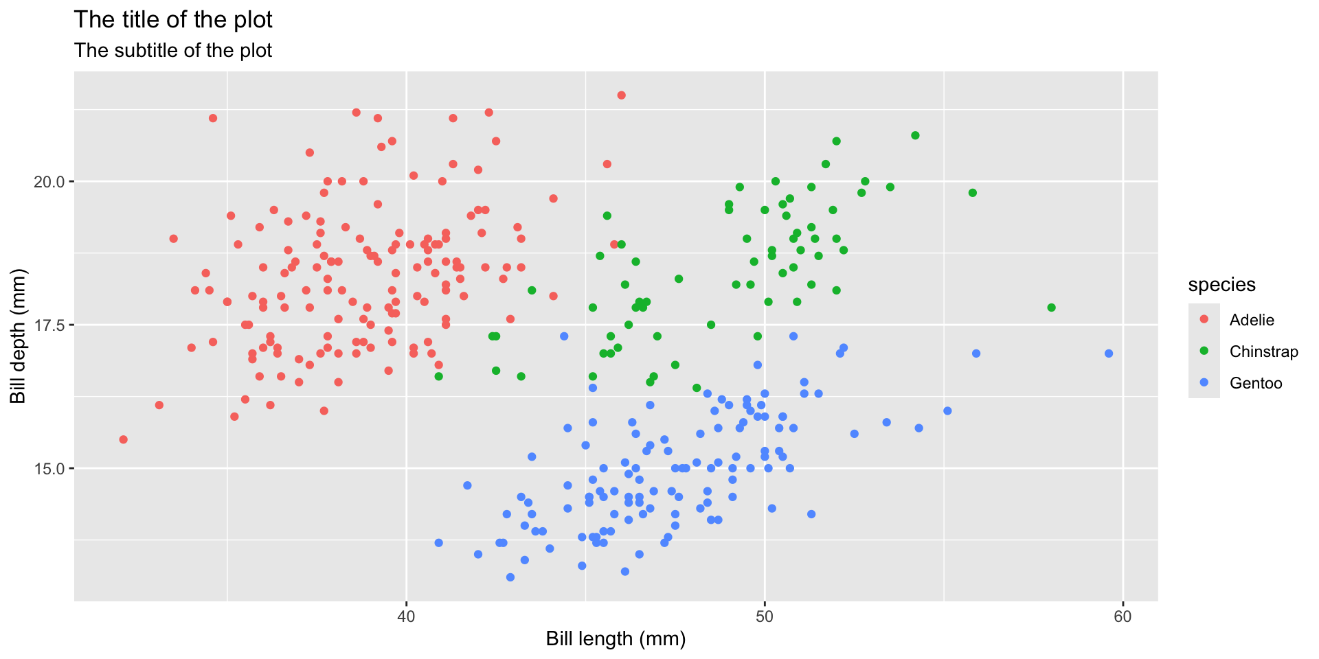
Write Labels

Task
Code
Output

Title of the plot
Subtitle of the plot with more information
Title of the x-axis
Title of the y-axis

ggplot(data = penguins,
       mapping = aes(x = bill_length_mm, y = bill_depth_mm)) +
  geom_point(aes(color = species)) +
  labs(
    title = "The title of the plot",
    subtitle = "The subtitle of the plot",
    x = "Bill length (mm)",
    y = "Bill depth (mm)"
  )

Different Shapes

Task
Code
Output

Each level of the factor/category can be shown using a different shape of different color.

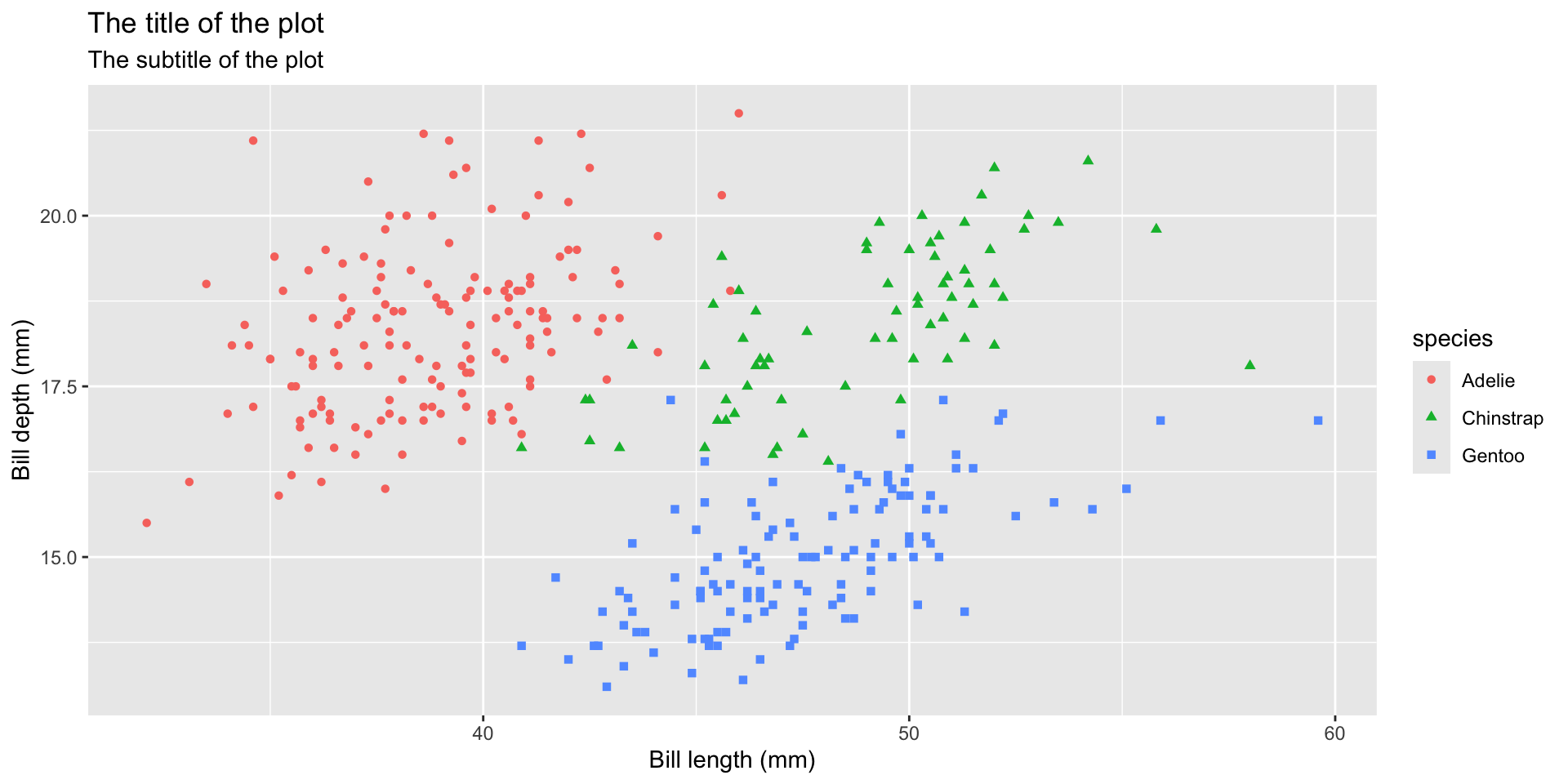
ggplot(data = penguins,
       mapping = aes(x = bill_length_mm, y = bill_depth_mm)) +
  geom_point(aes(color = species, shape = species)) +
  labs(
    title = "The title of the plot",
    subtitle = "The subtitle of the plot",
    x = "Bill length (mm)",
    y = "Bill depth (mm)"
  )

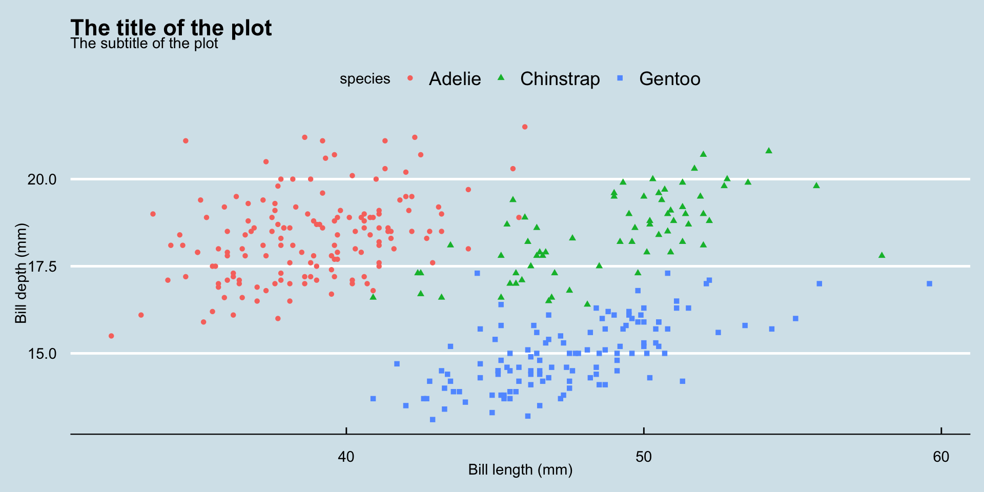
Various Themes

Task
Code
Output

Source: ggthemes

library(ggthemes)

ggplot(data = penguins,
       mapping = aes(x = bill_length_mm, y = bill_depth_mm)) +
  geom_point(aes(color = species, shape = species)) +
  labs(
    title = "The title of the plot",
    subtitle = "The subtitle of the plot",
    x = "Bill length (mm)",
    y = "Bill depth (mm)"
  ) +
  theme_economist()

Various Themes

Task
Code
Output

Source: ggthemes

library(ggthemes)

ggplot(data = penguins,
       mapping = aes(x = bill_length_mm, y = bill_depth_mm)) +
  geom_point(aes(color = species, shape = species)) +
  labs(
    title = "The title of the plot",
    subtitle = "The subtitle of the plot",
    x = "Bill length (mm)",
    y = "Bill depth (mm)"
  ) +
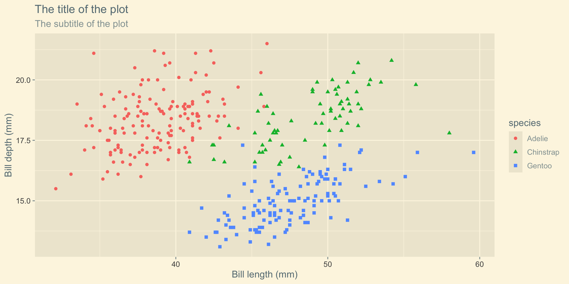
  theme_solarized_2()

Various Themes

Task
Code
Output

Source: ggthemes

library(ggthemes)

ggplot(data = penguins,
       mapping = aes(x = bill_length_mm, y = bill_depth_mm)) +
  geom_point(aes(color = species, shape = species)) +
  labs(
    title = "The title of the plot",
    subtitle = "The subtitle of the plot",
    x = "Bill length (mm)",
    y = "Bill depth (mm)"
  ) +
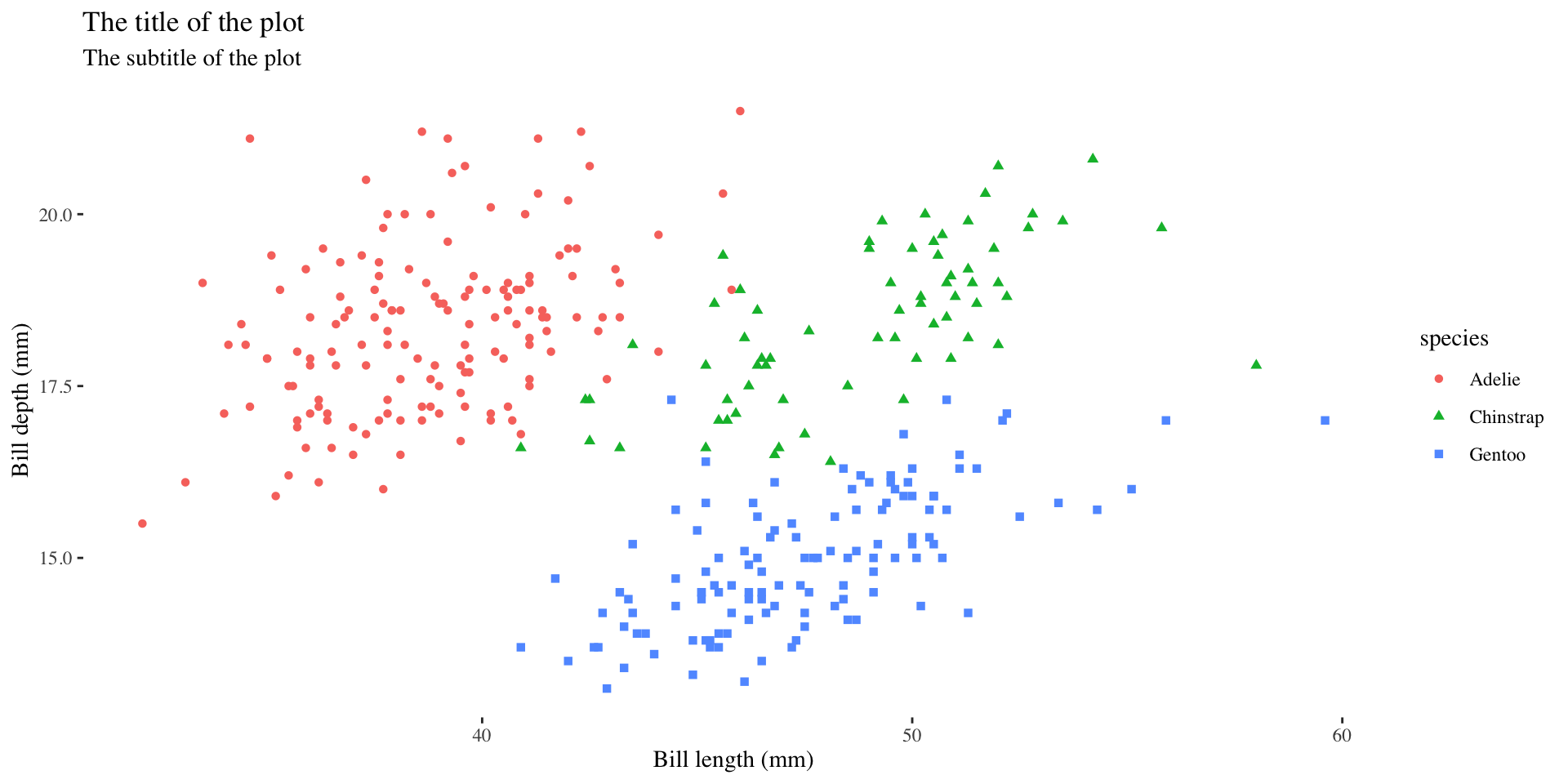
  theme_tufte()

Various Themes

Task
Code
Output

Source: ggthemes

library(ggthemes)

ggplot(data = penguins,
       mapping = aes(x = bill_length_mm, y = bill_depth_mm)) +
  geom_point(aes(color = species, shape = species)) +
  labs(
    title = "The title of the plot",
    subtitle = "The subtitle of the plot",
    x = "Bill length (mm)",
    y = "Bill depth (mm)"
  ) +
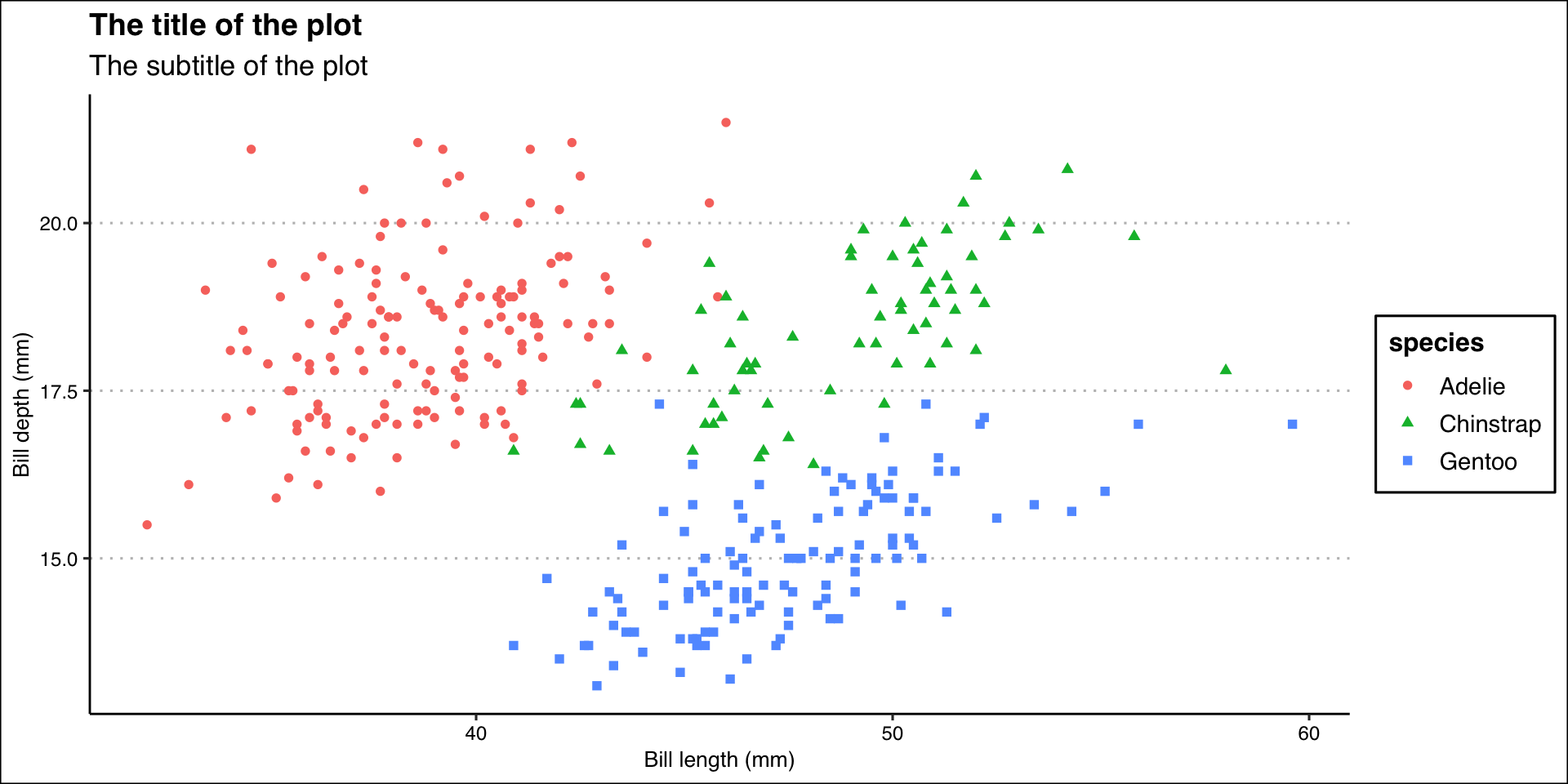
  theme_clean()

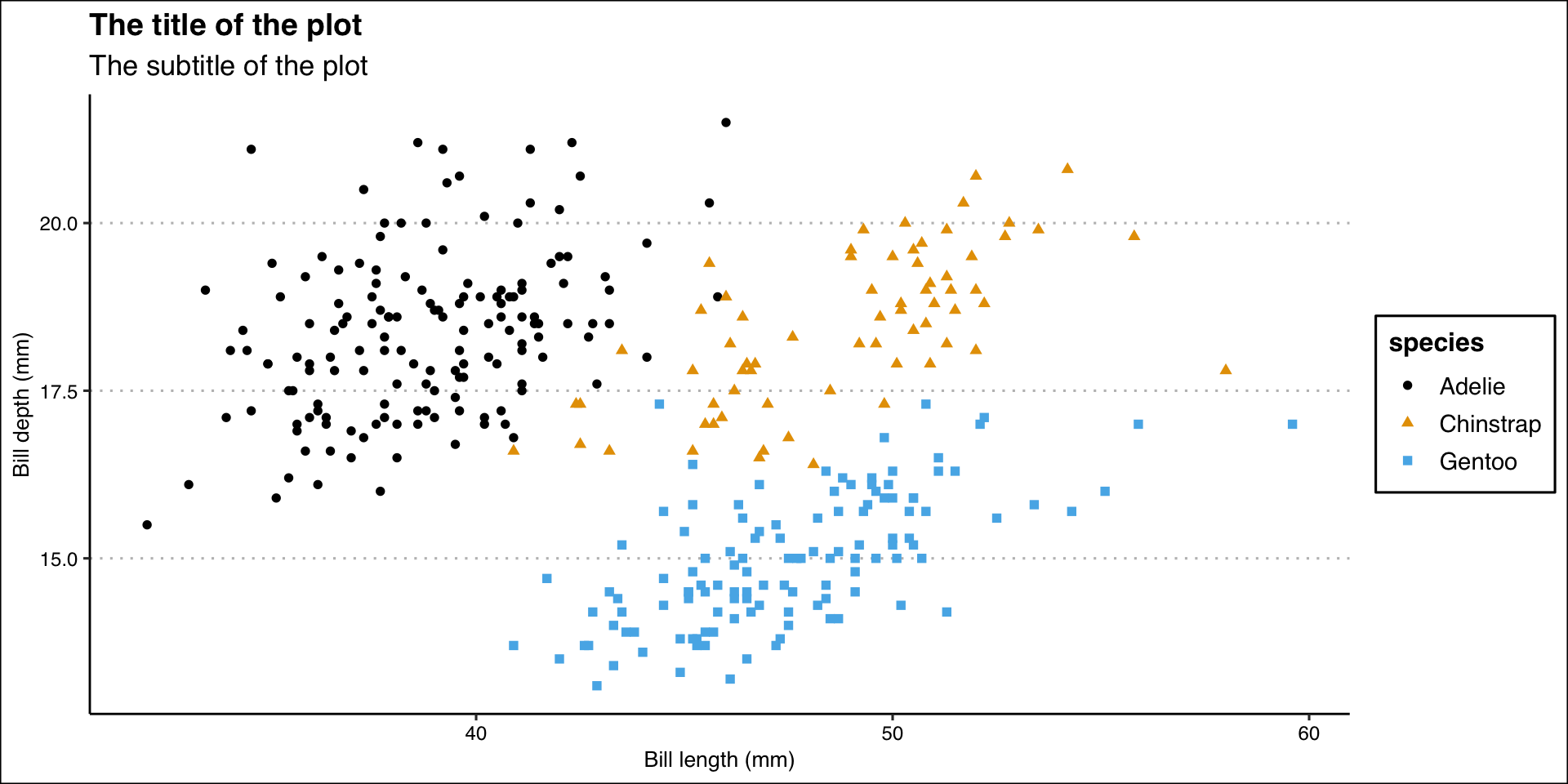
Color Palette

Task
Code
Output

R package ggthemes have function to use color scheme for colorblindness. Know more

ggplot(data = penguins,
       mapping = aes(x = bill_length_mm, y = bill_depth_mm)) +
  geom_point(aes(color = species, shape = species)) +
  labs(
    title = "The title of the plot",
    subtitle = "The subtitle of the plot",
    x = "Bill length (mm)",
    y = "Bill depth (mm)"
  ) +
  theme_clean() +
  scale_color_colorblind()

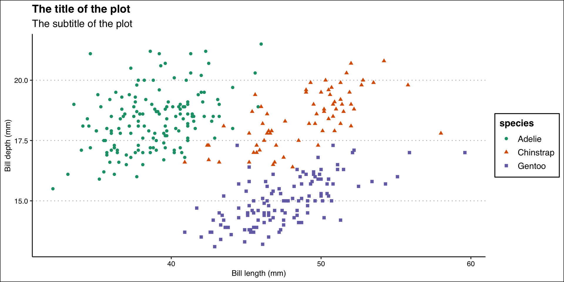
Color Palette

Task
Code
Output

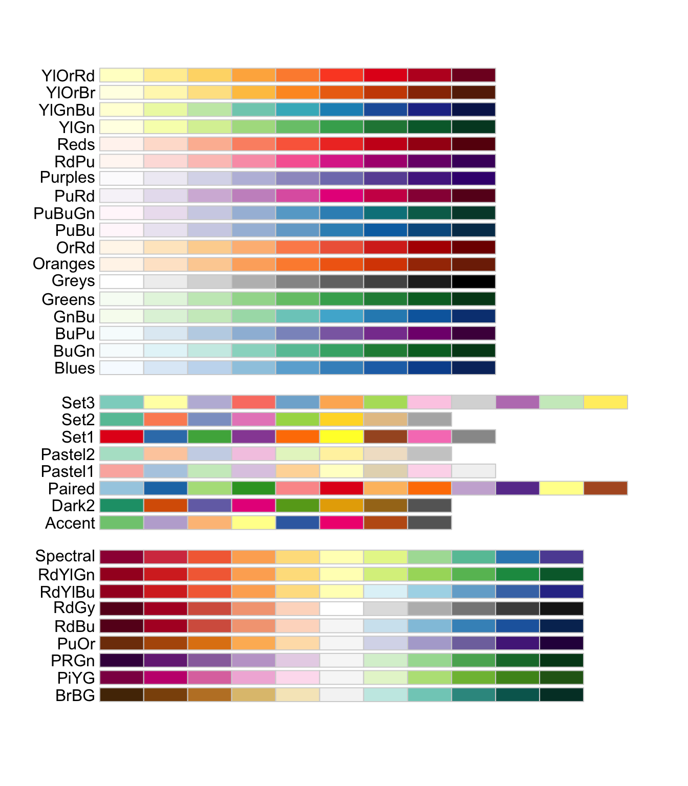
library(RColorBrewer)

ggplot(data = penguins,
       mapping = aes(x = bill_length_mm, y = bill_depth_mm)) +
  geom_point(aes(color = species, shape = species)) +
  labs(
    title = "The title of the plot",
    subtitle = "The subtitle of the plot",
    x = "Bill length (mm)",
    y = "Bill depth (mm)"
  ) +
  theme_clean() +
  scale_color_brewer(palette = "Dark2")

Color Palette

Task
Code
Output

library(wesanderson)

names(wes_palettes)

 [1] "BottleRocket1"     "BottleRocket2"     "Rushmore1"        
 [4] "Rushmore"          "Royal1"            "Royal2"           
 [7] "Zissou1"           "Zissou1Continuous" "Darjeeling1"      
[10] "Darjeeling2"       "Chevalier1"        "FantasticFox1"    
[13] "Moonrise1"         "Moonrise2"         "Moonrise3"        
[16] "Cavalcanti1"       "GrandBudapest1"    "GrandBudapest2"   
[19] "IsleofDogs1"       "IsleofDogs2"       "FrenchDispatch"   
[22] "AsteroidCity1"     "AsteroidCity2"     "AsteroidCity3"

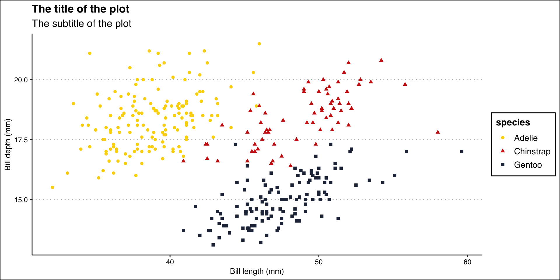
ggplot(data = penguins,
       mapping = aes(x = bill_length_mm, y = bill_depth_mm)) +
  geom_point(aes(color = species, shape = species)) +
  labs(
    title = "The title of the plot",
    subtitle = "The subtitle of the plot",
    x = "Bill length (mm)",
    y = "Bill depth (mm)"
  ) +
  theme_clean() +
  scale_color_manual(values = wes_palette("BottleRocket2", n = 3))

Export Plot

Task
Code
Output

Export/save plot as pdf, jpg or png file.

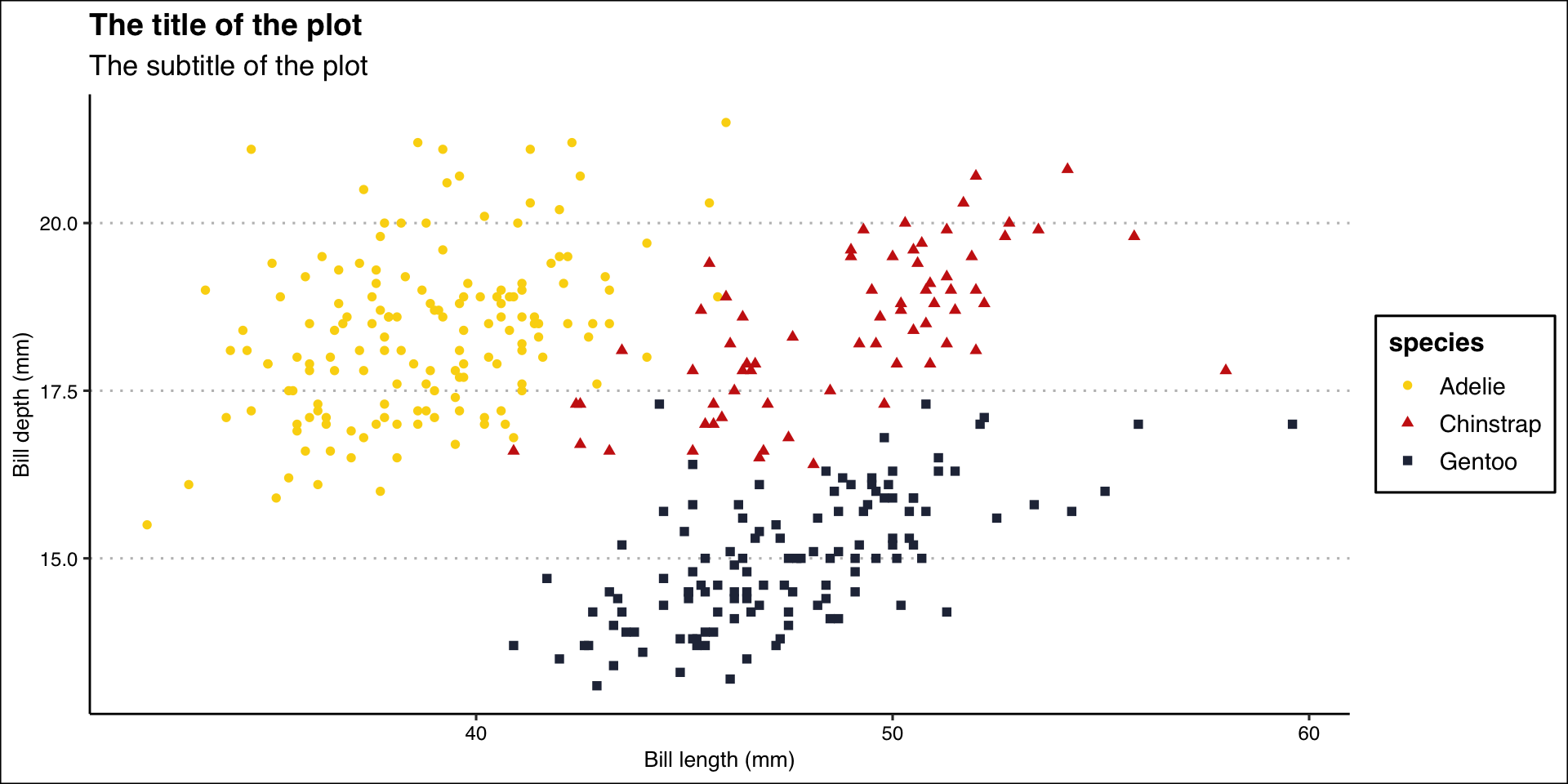
ggplot(data = penguins,
       mapping = aes(x = bill_length_mm, y = bill_depth_mm)) +
  geom_point(aes(color = species, shape = species)) +
  labs(
    title = "The title of the plot",
    subtitle = "The subtitle of the plot",
    x = "Bill length (mm)",
    y = "Bill depth (mm)"
  ) +
  theme_clean() +
  scale_color_manual(values = wes_palette("BottleRocket2", n = 3))

ggsave("penguins-plot.pdf")

🧑🏽‍💻👨🏽‍💻
Question & Answer

DataVisualisation

Data Visualization

Climate Spiral

The R Graph Gallery

Computational Art

Grammar of Graphics

Set-up

Know your Data

Ultimate Goal

ggplot2 Layers

Import Data

Map Variables Aesthetics

Add Geometric Shapes

Key Components are:

🧠 YOUR TURN

“Fill” Color

“Fill” Colors

“Fill” Colors vs “Color” Colors

📝 YOUR TURN

Plot A Continuous Variable

🧠 YOUR TURN

Two Continuous Variables

Geom Size

Geom Shape

📝 YOUR TURN

Plot A Factor & Factor

Plot A Factor & Continuous

A Factor & Two Cont. Variables

A Factor & Two Cont. Variables

Write Labels

Different Shapes

Various Themes

Various Themes

Various Themes

Various Themes

Color Palette

Color Palette

Color Palette

Color Palette

Export Plot

Data
Visualisation