Practice Sheet Day 5

SARA Statistics Winter School

Author

Dr. Ajay Koli

Published

July 29, 2025

1 Variables

We’ll simulate data to demonstrate the relationship between independent and dependent variables.

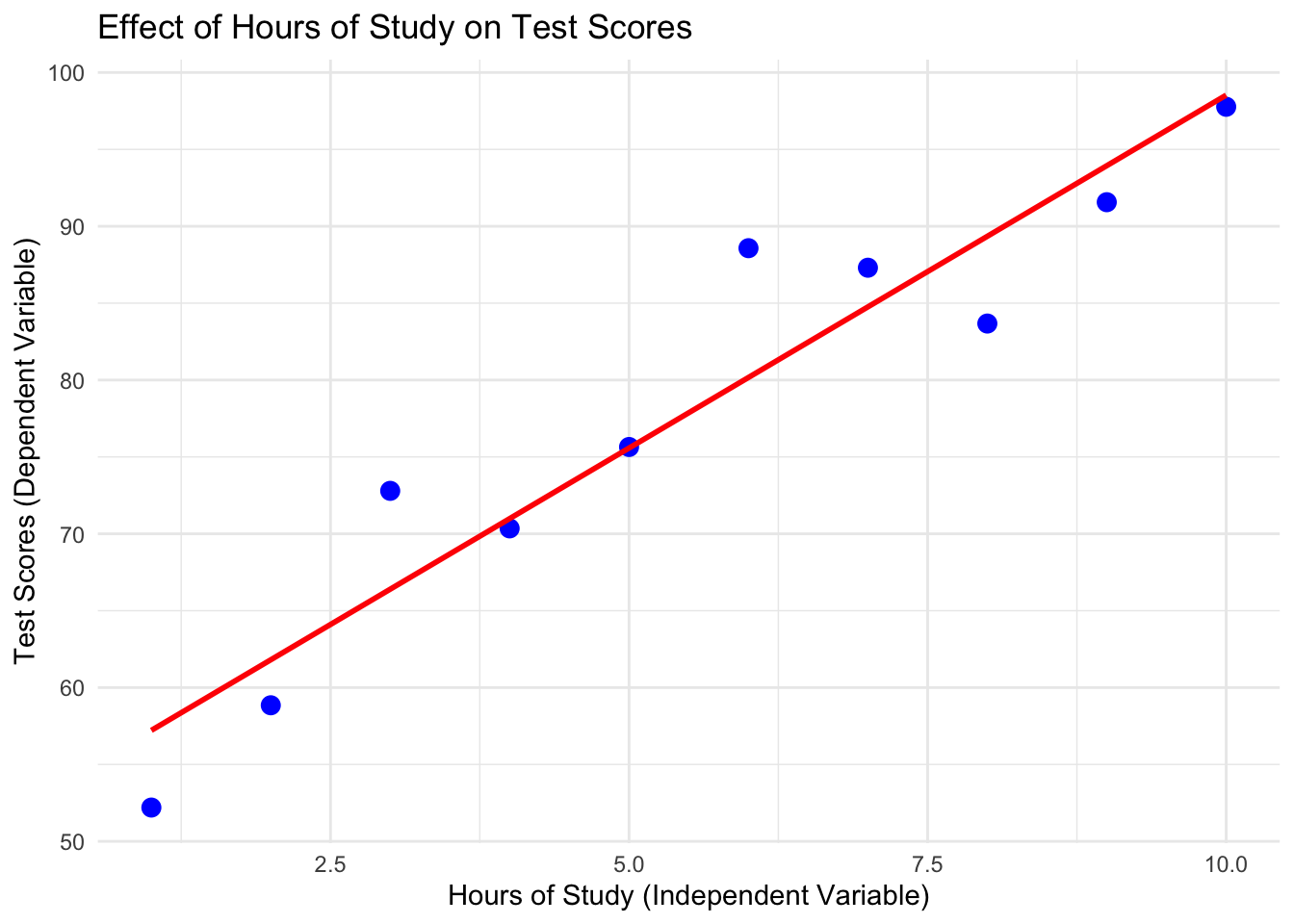
1.1 Example: Hours of Study and Test Scores

# Simulate data
set.seed(123)
hours_of_study <- c(1, 2, 3, 4, 5, 6, 7, 8, 9, 10) # Independent Variable
test_scores <- 50 + 5 * hours_of_study + rnorm(10, mean = 0, sd = 5) # Dependent Variable

# Combine into a data frame
data <- data.frame(Hours = hours_of_study, Scores = test_scores)

# Visualize the relationship
library(ggplot2)

ggplot(data, aes(x = Hours, y = Scores)) +
  geom_point(color = "blue", size = 3) +
  geom_smooth(method = "lm", se = FALSE, color = "red") +
  labs(
    title = "Effect of Hours of Study on Test Scores",
    x = "Hours of Study (Independent Variable)",
    y = "Test Scores (Dependent Variable)"
  ) +
  theme_minimal()

`geom_smooth()` using formula = 'y ~ x'

Interpretation of the Graph

X-axis (Independent Variable): Hours of study.
Y-axis (Dependent Variable): Test scores.
As hours of study increase, test scores generally increase, showing a positive relationship.

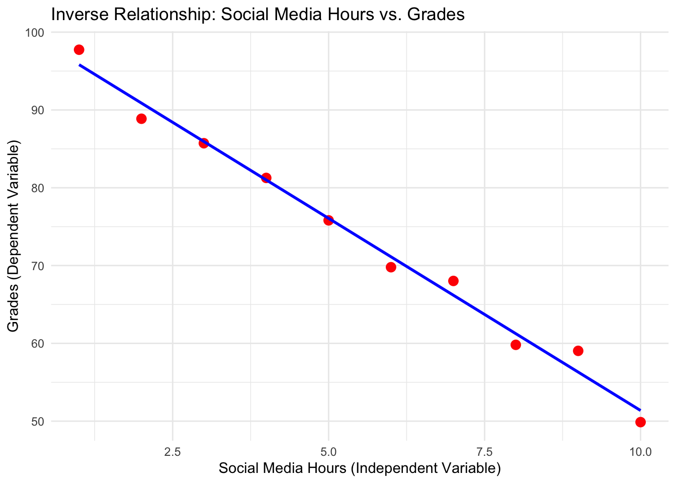
1.2 Inverse Relationship Example

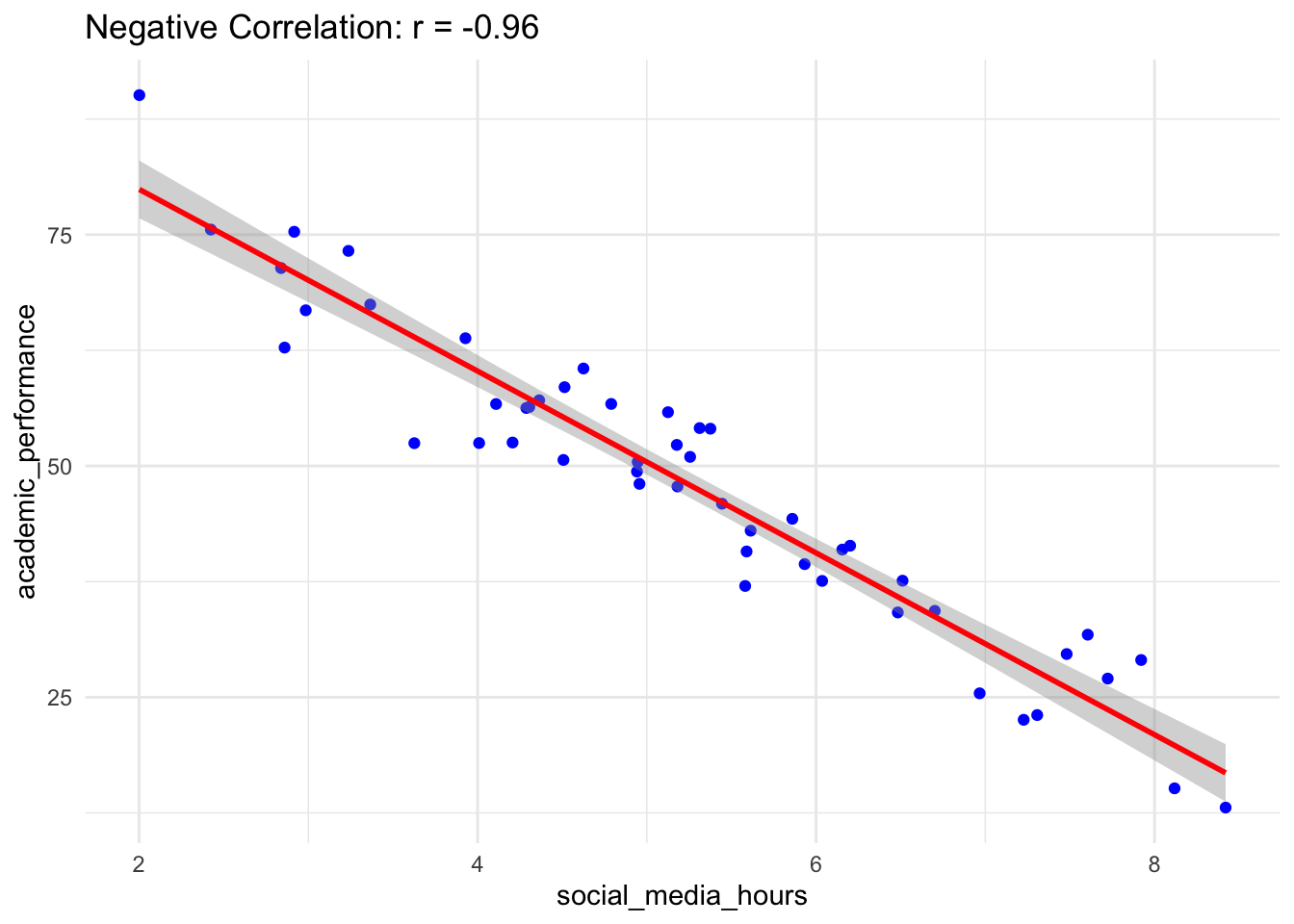
An inverse relationship occurs when one variable increases while the other decreases. For instance, the more time spent on social media, the lower the grades a student might achieve.

# Simulate data
set.seed(42)
social_media_hours <- seq(1, 10, by = 1)  # Independent Variable
grades <- 100 - 5 * social_media_hours + rnorm(10, mean = 0, sd = 2)  # Dependent Variable

# Combine into a data frame
inverse_data <- data.frame(SocialMediaHours = social_media_hours, Grades = grades)

# Visualize the inverse relationship
library(ggplot2)

ggplot(inverse_data, aes(x = SocialMediaHours, y = Grades)) +
  geom_point(color = "red", size = 3) +
  geom_smooth(method = "lm", se = FALSE, color = "blue") +
  labs(
    title = "Inverse Relationship: Social Media Hours vs. Grades",
    x = "Social Media Hours (Independent Variable)",
    y = "Grades (Dependent Variable)"
  ) +
  theme_minimal()

`geom_smooth()` using formula = 'y ~ x'

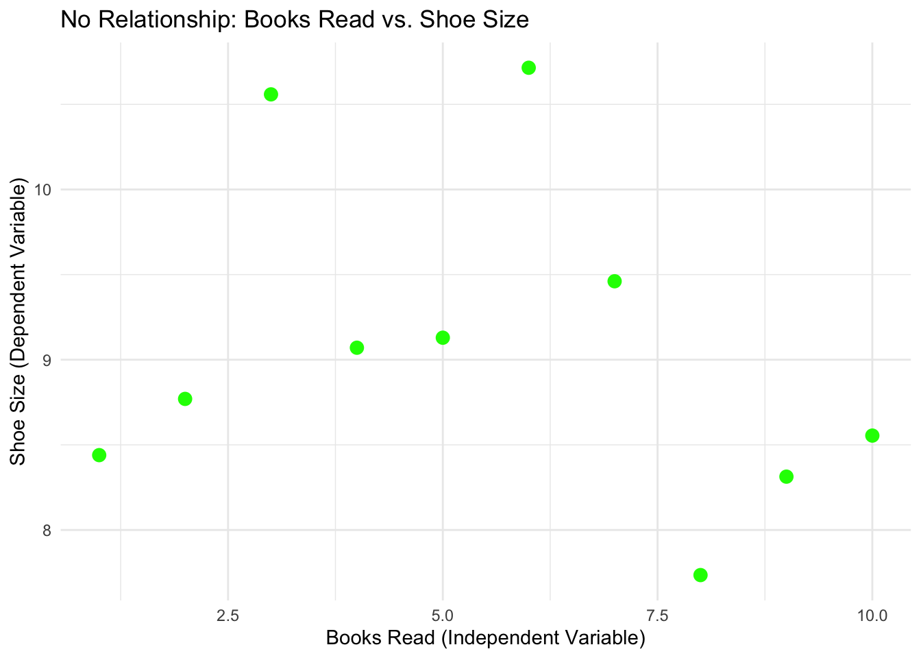
1.3 No-Relation Example

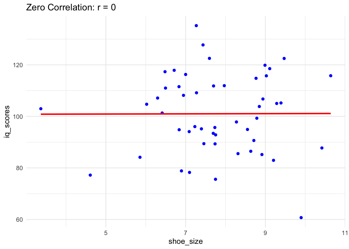
A no-relation scenario means that changes in one variable do not systematically affect the other. For instance, the number of books read by a person and their shoe size typically have no relationship.

# Simulate data
set.seed(123)
books_read <- seq(1, 10, by = 1)  # Independent Variable
shoe_size <- rnorm(10, mean = 9, sd = 1)  # Random data with no relation to books_read

# Combine into a data frame
no_relation_data <- data.frame(BooksRead = books_read, ShoeSize = shoe_size)

# Visualize the no-relation scenario
ggplot(no_relation_data, aes(x = BooksRead, y = ShoeSize)) +
  geom_point(color = "green", size = 3) +
  labs(
    title = "No Relationship: Books Read vs. Shoe Size",
    x = "Books Read (Independent Variable)",
    y = "Shoe Size (Dependent Variable)"
  ) +
  theme_minimal()

2 NHST

2.1 One-Sample t-Test

Scenario: A teacher claims that the average test score in a class is 70. You want to test if the actual average is different from 70.

$H_{0}$ : The mean test score is 70 ( $μ$ = 70).
$H_{a}$ : The mean test score is not 70 ( $μ \neq$ 70).

# Simulated data: Test scores of students
set.seed(123)
test_scores <- rnorm(30, mean = 72, sd = 5)

# Perform a one-sample t-test
t_test_result <- t.test(test_scores, mu = 70)

# Print the result
print(t_test_result)


    One Sample t-test

data:  test_scores
t = 1.9703, df = 29, p-value = 0.05842
alternative hypothesis: true mean is not equal to 70
95 percent confidence interval:
 69.93287 73.59610
sample estimates:
mean of x 
 71.76448

Interpretation:

If the p-value is less than 0.05, reject $H_{0}$ . This means the average test score is significantly different from 70.

2.2 Two-Sample t-Test

Scenario: Compare the average test scores of two groups: one that received tutoring and one that did not.

$H_{0}$ : The mean test scores the two groups are equal ( $μ_{1} = μ_{2}$ ).
$H_{a}$ : The mean test scores of the two groups are not equal ( $μ_{1} \neq μ_{2}$ ).

# Simulated data
set.seed(456)
group_A <- rnorm(30, mean = 75, sd = 5)  # Tutored group
group_B <- rnorm(30, mean = 70, sd = 5)  # Non-tutored group

# Perform a two-sample t-test
two_sample_test <- t.test(group_A, group_B, alternative = "two.sided")

# Print the result
print(two_sample_test)


    Welch Two Sample t-test

data:  group_A and group_B
t = 4.1181, df = 53.018, p-value = 0.0001344
alternative hypothesis: true difference in means is not equal to 0
95 percent confidence interval:
 2.758615 7.997380
sample estimates:
mean of x mean of y 
 76.15872  70.78072

Interpretation:

If the p-value is less than 0.05, reject $H_{0}$ . This indicates a significant difference between the two groups.

2.3 Chi-Square Test

Scenario: Test if there is an association between gender and preference for two types of beverages.

$H_{0}$ : Gender and beverage preference are independent.
$H - a$ : Gender and beverage preference are not independent.

# Simulated data
gender <- c("Male", "Male", "Female", "Female", "Male", "Female", "Male", "Female")
beverage <- c("Tea", "Coffee", "Tea", "Coffee", "Coffee", "Tea", "Coffee", "Tea")

# Create a contingency table
table_data <- table(gender, beverage)

# Perform a chi-square test
chi_sq_test <- chisq.test(table_data)

Warning in chisq.test(table_data): Chi-squared approximation may be incorrect

# Print the result
print(chi_sq_test)


    Pearson's Chi-squared test with Yates' continuity correction

data:  table_data
X-squared = 0.5, df = 1, p-value = 0.4795

Interpretation:

If the p-value is less than 0.05, reject $H_{0}$ . This suggests that gender and beverage preference are associated.

2.4 ANOVA (Analysis of Variance)

Scenario: Test if three different fertilizers lead to different crop yields.

$H_{0}$ : The mean yields are the same for all fertilizers ( $μ_{1} = μ_{2} = μ_{3}$ ).
$H_{a}$ : At least one fertilizer leads to a different mean yield

# Simulated data
set.seed(789)
fertilizer <- factor(rep(c("Fert1", "Fert2", "Fert3"), each = 10))
yield <- c(rnorm(10, mean = 50, sd = 5), rnorm(10, mean = 55, sd = 5), rnorm(10, mean = 60, sd = 5))

# Perform ANOVA
anova_result <- aov(yield ~ fertilizer)
summary(anova_result)

            Df Sum Sq Mean Sq F value   Pr(>F)    
fertilizer   2  567.3   283.7   21.16 2.96e-06 ***
Residuals   27  361.9    13.4                     
---
Signif. codes:  0 '***' 0.001 '**' 0.01 '*' 0.05 '.' 0.1 ' ' 1

Interpretation:

If the p-value is less than 0.05, reject $H_{0}$ . This means at least one fertilizer has a significantly different effect.

2.5 Correlation Test

Scenario: Test if there is a significant correlation between hours studied and test scores.

$H_{0}$ : There is no correlation between hours studied and test scores ( $r = 0$ ).
$H_{a}$ : There is a correlation between hours studied and test scores ( $r \neq 0$ ).

# Simulated data
set.seed(101)
hours_studied <- rnorm(50, mean = 5, sd = 2)
test_scores <- hours_studied * 10 + rnorm(50, mean = 50, sd = 10)

# Perform correlation test
cor_test <- cor.test(hours_studied, test_scores)

# Print the result
print(cor_test)


    Pearson's product-moment correlation

data:  hours_studied and test_scores
t = 14.407, df = 48, p-value < 2.2e-16
alternative hypothesis: true correlation is not equal to 0
95 percent confidence interval:
 0.8314306 0.9430071
sample estimates:
      cor 
0.9012134

Interpretation:

If the p-value is less than 0.05, reject $H_{0}$ . This indicates a significant correlation.

3 Correlation

3.1 Positive Correlation

When one variable increases, the other variable also increases.

Example: Height and weight of individuals.

# Simulated data
set.seed(123)
height <- rnorm(50, mean = 160, sd = 10)  # Heights in cm
weight <- height * 0.5 + rnorm(50, mean = 50, sd = 5)  # Weights in kg

# Calculate correlation
correlation_positive <- cor(height, weight)

# Visualization
library(ggplot2)
ggplot(data.frame(height, weight), aes(x = height, y = weight)) +
  geom_point(color = "blue") +
  geom_smooth(method = "lm", color = "red") +
  ggtitle(paste("Positive Correlation: r =", round(correlation_positive, 2))) +
  theme_minimal()

`geom_smooth()` using formula = 'y ~ x'

3.2 Negative Correlation

When one variable increases, the other variable decreases.

Example: Hours spent on social media vs. academic performance.

# Simulated data
set.seed(456)
social_media_hours <- rnorm(50, mean = 5, sd = 1.5)
academic_performance <- 100 - (social_media_hours * 10) + rnorm(50, mean = 0, sd = 5)

# Calculate correlation
correlation_negative <- cor(social_media_hours, academic_performance)

# Visualization
ggplot(data.frame(social_media_hours, academic_performance), aes(x = social_media_hours, y = academic_performance)) +
  geom_point(color = "blue") +
  geom_smooth(method = "lm", color = "red") +
  ggtitle(paste("Negative Correlation: r =", round(correlation_negative, 2))) +
  theme_minimal()

`geom_smooth()` using formula = 'y ~ x'

3.3 Zero Correlation

No relationship exists between the variables.

Example: Shoe size and IQ.

# Simulated data
set.seed(789)
shoe_size <- rnorm(50, mean = 8, sd = 1.5)
iq_scores <- rnorm(50, mean = 100, sd = 15)

# Calculate correlation
correlation_zero <- cor(shoe_size, iq_scores)

# Visualization
ggplot(data.frame(shoe_size, iq_scores), aes(x = shoe_size, y = iq_scores)) +
  geom_point(color = "blue") +
  geom_smooth(method = "lm", color = "red", se = FALSE) +
  ggtitle(paste("Zero Correlation: r =", round(correlation_zero, 2))) +
  theme_minimal()

`geom_smooth()` using formula = 'y ~ x'

3.4 Perfect Positive Correlation

Both variables move together with the same ratio.

Example: Temperature in Celsius and Fahrenheit.

# Simulated data
celsius <- seq(0, 100, by = 2)
fahrenheit <- celsius * 1.8 + 32

# Calculate correlation
correlation_perfect_positive <- cor(celsius, fahrenheit)

# Visualization
ggplot(data.frame(celsius, fahrenheit), aes(x = celsius, y = fahrenheit)) +
  geom_point(color = "blue") +
  geom_smooth(method = "lm", color = "red", se = FALSE) +
  ggtitle(paste("Perfect Positive Correlation: r =", round(correlation_perfect_positive, 2))) +
  theme_minimal()

`geom_smooth()` using formula = 'y ~ x'

3.5 Non-Linear Correlation

The relationship between variables is non-linear.

Example: Age and happiness level.

# Simulated data
set.seed(101)
age <- seq(1, 80, length.out = 100)
happiness <- -0.02 * (age - 40)^2 + 80 + rnorm(100, sd = 3)

# Visualization
ggplot(data.frame(age, happiness), aes(x = age, y = happiness)) +
  geom_point(color = "blue") +
  geom_smooth(method = "loess", color = "red") +
  ggtitle("Non-Linear Correlation") +
  theme_minimal()

`geom_smooth()` using formula = 'y ~ x'

3.6 Perfect Negative Correlation

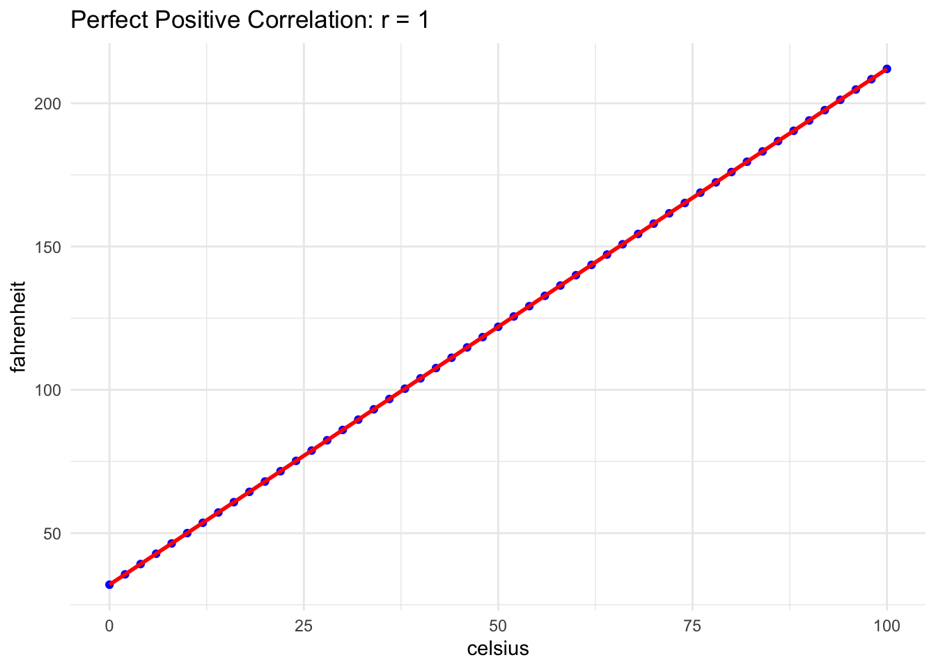
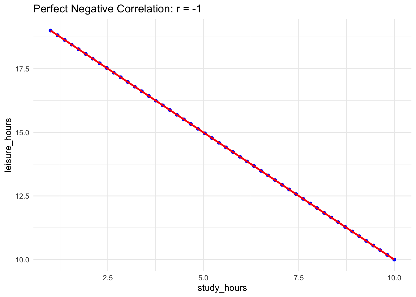
One variable increases while the other decreases in a perfect ratio.

Example: Number of hours spent studying and hours spent on leisure.

# Simulated data
study_hours <- seq(1, 10, length.out = 50)
leisure_hours <- 20 - study_hours

# Calculate correlation
correlation_perfect_negative <- cor(study_hours, leisure_hours)

# Visualization
ggplot(data.frame(study_hours, leisure_hours), aes(x = study_hours, y = leisure_hours)) +
  geom_point(color = "blue") +
  geom_smooth(method = "lm", color = "red", se = FALSE) +
  ggtitle(paste("Perfect Negative Correlation: r =", round(correlation_perfect_negative, 2))) +
  theme_minimal()

`geom_smooth()` using formula = 'y ~ x'

4 Regression

4.1 Simple Linear Regression

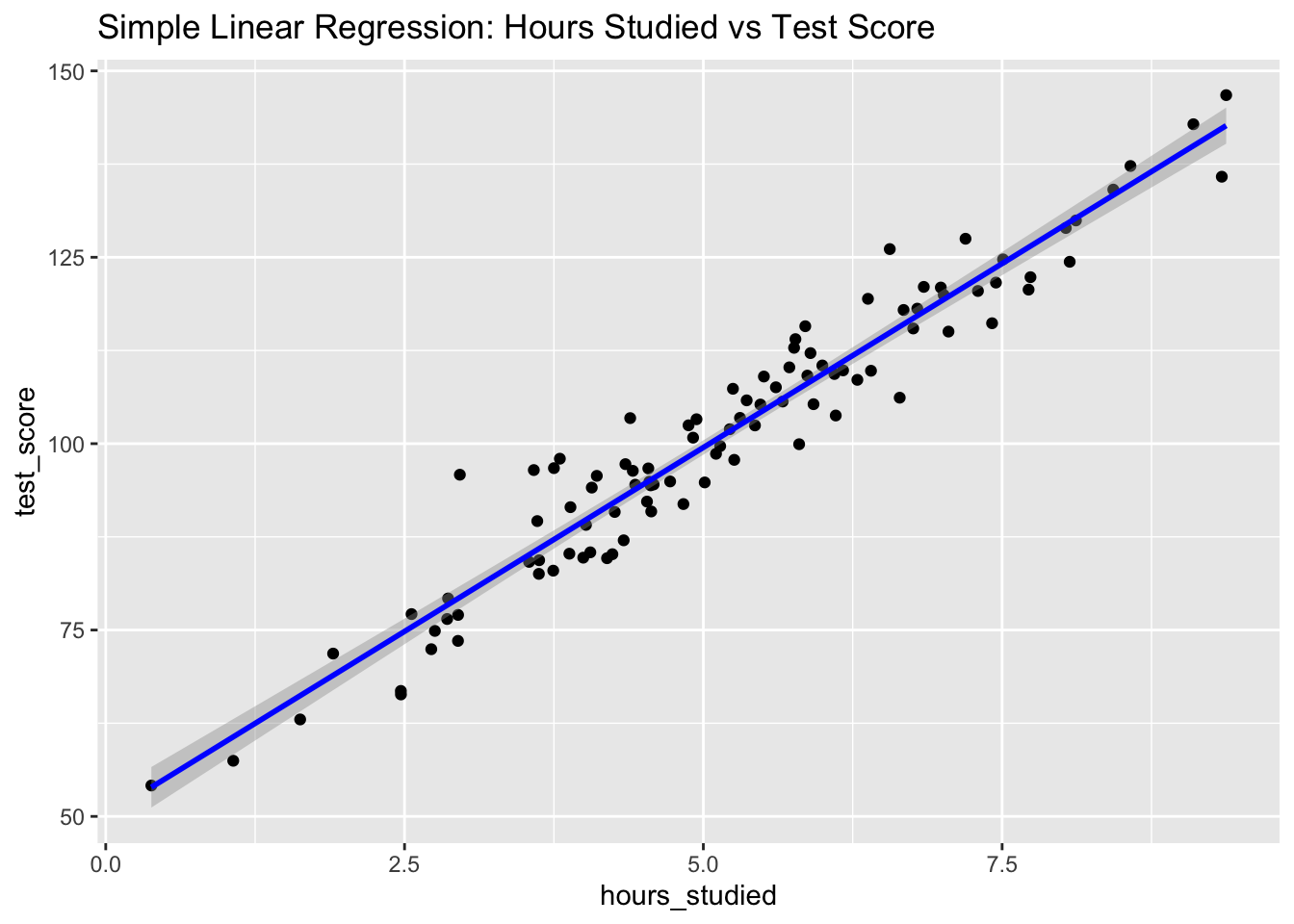
Scenario: Predict a student’s test score based on the number of hours studied.

# Simulated data
set.seed(123)
hours_studied <- rnorm(100, mean = 5, sd = 2)
test_score <- 50 + 10 * hours_studied + rnorm(100, mean = 0, sd = 5)

# Data preparation
data_simple <- data.frame(hours_studied, test_score)

# Fit Simple Linear Regression
model_simple <- lm(test_score ~ hours_studied, data = data_simple)

# Summary of the model
summary(model_simple)


Call:
lm(formula = test_score ~ hours_studied, data = data_simple)

Residuals:
    Min      1Q  Median      3Q     Max 
-9.5367 -3.4175 -0.4375  2.9032 16.4520 

Coefficients:
              Estimate Std. Error t value Pr(>|t|)    
(Intercept)    50.1419     1.4669   34.18   <2e-16 ***
hours_studied   9.8688     0.2672   36.94   <2e-16 ***
---
Signif. codes:  0 '***' 0.001 '**' 0.01 '*' 0.05 '.' 0.1 ' ' 1

Residual standard error: 4.854 on 98 degrees of freedom
Multiple R-squared:  0.933, Adjusted R-squared:  0.9323 
F-statistic:  1364 on 1 and 98 DF,  p-value: < 2.2e-16

# Visualization
library(ggplot2)
ggplot(data_simple, aes(x = hours_studied, y = test_score)) +
  geom_point() +
  geom_smooth(method = "lm", color = "blue") +
  ggtitle("Simple Linear Regression: Hours Studied vs Test Score")

`geom_smooth()` using formula = 'y ~ x'

Intercept: The average test score when hours studied = 0.
Coefficient (hours_studied): For each additional hour studied, test score increases by approximately the coefficient value.
R-squared: Indicates how much of the variability in test scores is explained by hours studied. A value close to 1 suggests a strong relationship.
P-value: If significant (typically p < 0.05), hours studied significantly predicts test scores.

Interpretation:

Students who study more hours tend to achieve higher test scores. The model can explain a substantial portion of the variation in scores through study time.

4.2 Multiple Linear Regression

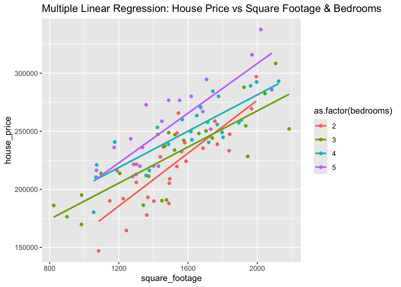
Scenario: Predict house price based on square footage and number of bedrooms.

# Simulated data
set.seed(456)
square_footage <- rnorm(100, mean = 1500, sd = 300)
bedrooms <- sample(2:5, 100, replace = TRUE)
house_price <- 50000 + 100 * square_footage + 10000 * bedrooms + rnorm(100, mean = 0, sd = 20000)

# Data preparation
data_multiple <- data.frame(square_footage, bedrooms, house_price)

# Fit Multiple Linear Regression
model_multiple <- lm(house_price ~ square_footage + bedrooms, data = data_multiple)

# Summary of the model
summary(model_multiple)


Call:
lm(formula = house_price ~ square_footage + bedrooms, data = data_multiple)

Residuals:
   Min     1Q Median     3Q    Max 
-41628 -14765   1413  14674  43071 

Coefficients:
                Estimate Std. Error t value Pr(>|t|)    
(Intercept)    61626.704  11546.090   5.337 6.19e-07 ***
square_footage    89.182      6.481  13.760  < 2e-16 ***
bedrooms       11610.356   1754.323   6.618 2.01e-09 ***
---
Signif. codes:  0 '***' 0.001 '**' 0.01 '*' 0.05 '.' 0.1 ' ' 1

Residual standard error: 19360 on 97 degrees of freedom
Multiple R-squared:  0.7134,    Adjusted R-squared:  0.7075 
F-statistic: 120.7 on 2 and 97 DF,  p-value: < 2.2e-16

# Visualization
ggplot(data_multiple, aes(x = square_footage, y = house_price, color = as.factor(bedrooms))) +
  geom_point() +
  geom_smooth(method = "lm", aes(group = bedrooms), se = FALSE) +
  ggtitle("Multiple Linear Regression: House Price vs Square Footage & Bedrooms")

`geom_smooth()` using formula = 'y ~ x'

Intercept: Baseline house price when square footage and bedrooms are 0.
Coefficients: Each unit increase in square footage or additional bedroom increases house price by the respective coefficient.
R-squared: Shows the proportion of variance in house price explained by square footage and bedrooms.

Interpretation:

Larger homes (in square footage) and more bedrooms are associated with higher house prices. Both variables are significant predictors, but additional bedrooms might have a stronger influence.

4.3 Time Series Regression

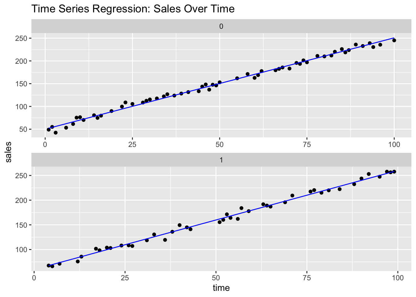
Scenario: Predict sales based on time trends and promotions.

# Simulated data
set.seed(303)
time <- 1:100
promotions <- sample(0:1, 100, replace = TRUE)
sales <- 50 + 2 * time + 10 * promotions + rnorm(100, mean = 0, sd = 5)

# Data preparation
data_time <- data.frame(time, promotions, sales)

# Fit Time Series Regression
model_time <- lm(sales ~ time + promotions, data = data_time)

# Summary of the model
summary(model_time)


Call:
lm(formula = sales ~ time + promotions, data = data_time)

Residuals:
     Min       1Q   Median       3Q      Max 
-13.7319  -3.2999   0.0154   3.7220  12.5617 

Coefficients:
            Estimate Std. Error t value Pr(>|t|)    
(Intercept) 50.05265    1.11623  44.841  < 2e-16 ***
time         2.00671    0.01785 112.450  < 2e-16 ***
promotions   9.47772    1.04050   9.109 1.13e-14 ***
---
Signif. codes:  0 '***' 0.001 '**' 0.01 '*' 0.05 '.' 0.1 ' ' 1

Residual standard error: 5.147 on 97 degrees of freedom
Multiple R-squared:  0.9925,    Adjusted R-squared:  0.9923 
F-statistic:  6413 on 2 and 97 DF,  p-value: < 2.2e-16

# Visualization
ggplot(data_time, aes(x = time, y = sales)) +
  geom_point() +
  geom_line(aes(y = predict(model_time)), color = "blue") +
  facet_wrap(~promotions, scales = "free", ncol = 1) +
  ggtitle("Time Series Regression: Sales Over Time")

Time Coefficient: Represents the trend over time.
Promotions Coefficient: Indicates the additional impact of running a promotion on sales.
R-squared: Measures how well time and promotions explain sales variability.

Interpretation:

Sales increase over time, possibly due to market growth or product popularity. Promotions have a significant positive impact on sales, validating their effectiveness.